Introduction

In this document we show how to:

Fit an SPiCT biomass dynamic model to the available data,
Condition FLBEIA using:

The output of SPiCT,
Red mullet’s life-history traits,

Test the performance of different harvest control rules in FLBEIA.

The first part of the tutorial deals with the analysis of the data to fit SPiCT and the process of finding an acceptable fit. It is not part of the data-poor tutorial per se. However we have included it in as part of the document to show how to fit the biomass dynamic model used later on to generate the initial random population.

and to condition and run FLBEIA is shown to demonstrate how to use them. First Spict is used to obtain the best assessment possible using the data available. Then using this fit and making use of the variance-covariance matrix estimated by the model a random population is obtained to condition FLBEIA. Alternatively, FLBEIA is conditioned using life-history traints and different hypothesis about its status in the initial year of the simulation and productivity. Finally FLBEIA is run using different harvest control rules (HCRs).

To start the R session, load SPicT, FLBEIA and the rest of the packages neccesary to run this tutorial. FLCore and FLFLeets are automatically loaded with FLBEIA.

The Case Study: Stripped Red Mullet in the Bay of Biscay

Stripped Red Mullet (Mullus surmuletus) in Bay of Biscay has no analytical assessment and it is not subject to the European TAC and quota system. It is mainly caught by France followed by Spain. The annual total catch is around 2000 tons. The stock is assessed in WGBIE (ICSE, 2017).

Data

The total catch time series data used in this analysis was taken from WGBIE report (ICES, 2017) and the EVHOE abundance index time series was provided by Ifremer.

Total catch data is available since 1975. In 1999 France did not report any data. As France is the main contributor to the total catch, the 1999 catch data was not included in the analysis.

The abundance index is available since 1997. In provides an estimation of the biomass together with a coefficient of variation.

In all the areas the catch shows an increasing trend since the begining of the series but in the last two years, 2013 and 2014, there has been a sharp decrease in the catches (see the figure below).

Catch time series by area.

The abundance index, in the figure below, does not show any clear trend. In 2001 and from 2003 to 2005 the observed values were well above the historical mean. In 2006 the index decreased sharply and in the last three years the values are among the lowest in the series.

EVHOE abundance index. Shaded area corresponds with two times the annual standard deviation of the index.

Initial SPiCT fit to the data.

The data used is stored in two data frames, ‘catch’ and ‘evhoe’. First we used these data frames to create a list with the shape required by SPiCT. We use the ‘check.inp’ function from SPiCT library to check that the data is right.

murDat <- list(obsC  = catch[,'area_total'],
               timeC = catch[,'year'],
               obsI  = evhoe[,'biomass'],
               timeI  = evhoe[,'year'])

murInp <- check.inp(murDat)

Removing zero, negative, and NAs in  C  series

murInp

Catch observations:
 [1] 1975 1976 1977 1978 1979 1980 1981 1982 1983 1984 1985 1986 1987 1988 1989
[16] 1990 1991 1992 1993 1994 1995 1996 1997 1998 2000 2001 2002 2003 2004 2005
[31] 2006 2007 2008 2009 2010 2011 2012 2013 2014
 [1] 1074 1854 1022  660  636  875  581  746 1180 1146 1319 1094 1335 1219 1137
[16] 1351 1480 1299 1161 1118 1099 1681 1628 1398 1955 2163 1730 2061 2881 2786
[31] 2819 2949 2313 2506 2753 2781 2149 1514 1402
Index observations:
[[1]]
 [1] 1997 1998 1999 2000 2001 2002 2003 2004 2005 2006 2007 2008 2009 2010 2011
[16] 2012 2013 2014

[[1]]
 [1]  188164.75  116595.14  117908.28  232345.48 1025351.89  275582.63
 [7] 1178844.41  756444.08 1345271.32  300872.56  336002.51  756698.89
[13]  324394.88  354774.49  648639.86   77729.27  173458.36  115474.63

Fit SPiCT model using the default settings and show the numeric output.

 mur_spict <- fit.spict(murInp)
 capture.output(summary(mur_spict))

 [1] "Convergence: 0  MSG: relative convergence (4)"                      
 [2] "Objective function at optimum: 24.9401239"                          
 [3] "Euler time step (years):  1/16 or 0.0625"                           
 [4] "Nobs C: 39,  Nobs I1: 18"                                           
 [5] ""                                                                   
 [6] "Priors"                                                             
 [7] "     logn  ~  dnorm[log(2), 2^2]"                                   
 [8] " logalpha  ~  dnorm[log(1), 2^2]"                                   
 [9] "  logbeta  ~  dnorm[log(1), 2^2]"                                   
[10] ""                                                                   
[11] "Model parameter estimates w 95% CI "                                
[12] "            estimate        cilow        ciupp    log.est  "        
[13] " alpha     7.7405185    0.9084707 6.595218e+01  2.0464687  "        
[14] " beta      0.1074761    0.0162522 7.107428e-01 -2.2304864  "        
[15] " r         0.9021157    0.4166625 1.953170e+00 -0.1030125  "        
[16] " rc        3.0999586    1.8848049 5.098535e+00  1.1313887  "        
[17] " rold      2.1582637    0.6779162 6.871207e+00  0.7693041  "        
[18] " m      2561.8260706 2432.0507159 2.698526e+03  7.8484756  "        
[19] " K      6033.9414167 3132.7337462 1.162194e+04  8.7051557  "        
[20] " q       399.2680789  258.1679013 6.174857e+02  5.9896331  "        
[21] " n         0.5820179    0.4405863 7.688501e-01 -0.5412541  "        
[22] " sdb       0.0711700    0.0083360 6.076269e-01 -2.6426843  "        
[23] " sdf       0.3335386    0.2510202 4.431835e-01 -1.0979967  "        
[24] " sdi       0.5508925    0.3947977 7.687040e-01 -0.5962156  "        
[25] " sdc       0.0358474    0.0058437 2.199002e-01 -3.3284830  "        
[26] " "                                                                  
[27] "Deterministic reference points (Drp)"                               
[28] "          estimate        cilow       ciupp   log.est  "            
[29] " Bmsyd 1652.813108 1006.5694231 2713.962006 7.4102340  "            
[30] " Fmsyd    1.549979    0.9424025    2.549267 0.4382416  "            
[31] " MSYd  2561.826071 2432.0507159 2698.526298 7.8484756  "            
[32] "Stochastic reference points (Srp)"                                  
[33] "         estimate        cilow       ciupp   log.est rel.diff.Drp  "
[34] " Bmsys 1655.45136 1019.4292309 2688.287854 7.4118290  0.001593678  "
[35] " Fmsys    1.54423    0.9522525    2.504215 0.4345252 -0.003723267  "
[36] " MSYs  2556.41241 2430.4846142 2688.864748 7.8463602 -0.002117680  "
[37] ""                                                                   
[38] "States w 95% CI (inp$msytype: s)"                                   
[39] "                   estimate       cilow       ciupp   log.est  "    
[40] " B_2014.00      218.1468527 156.7649995 303.5629731  5.385168  "    
[41] " F_2014.00        6.5200586   4.9165639   8.6465191  1.874883  "    
[42] " B_2014.00/Bmsy   0.1317748   0.0885892   0.1960128 -2.026661  "    
[43] " F_2014.00/Fmsy   4.2222076   2.9365271   6.0707894  1.440358  "    
[44] ""                                                                   
[45] "Predictions w 95% CI (inp$msytype: s)"                              
[46] "                  prediction       cilow       ciupp   log.est  "   
[47] " B_2015.00       213.0671013  79.8428427  568.586841  5.361607  "   
[48] " F_2015.00         6.5452358   3.1869139   13.442507  1.878737  "   
[49] " B_2015.00/Bmsy    0.1287063   0.0474129    0.349384 -2.050222  "   
[50] " F_2015.00/Fmsy    4.2385116   2.0140736    8.919724  1.444212  "   
[51] " Catch_2015.00  1401.4888698 872.7834599 2250.467776  7.245290  "   
[52] " E(B_inf)        213.1470534          NA          NA  5.361982  "

Plot the estimated biomass, absolute and relative, using the functions available in the package. Until the late 1990 the estimated biomass was very low. Then it started increasing until reaching the maximum in 2004. Afterwards it showed a decreasing trend. The biomass has been above Bmsy only in five years around 2004.

 par(mfrow = c(1,2))
 plotspict.bbmsy(mur_spict, qlegend = FALSE)
 plotspict.biomass(mur_spict, qlegend = FALSE)

Relative and Absolute Biomasses estimated by SPiCT. Horizontal line correspond with the biomass level at MSY.

Now plot the fishing mortality using the plotspict function. The fishing mortality has been above Fmsy in the whole time series. In the begining of the series the fishing mortality level was very high.

 par(mfrow = c(1,2))
 plotspict.f(mur_spict, qlegend = FALSE)
 plotspict.ffmsy(mur_spict, qlegend = FALSE)

Relative and Absolute fishing mortalities estimated by SPiCT. Horizontal line correspond with the MSY fishing mortality level.

The uncertainty estimated by the model around the catch is very small.

 plotspict.catch(mur_spict, qlegend = FALSE)

Catch estimated by SPiCT. The horizontal line corresponds with the MSY.

A sensitivity analysis to the starting values was performed. The results converged to two different data sets with more or less the same probability. The one shown above and an alternative case which had very wide confidence intervals. Another excercise was done fixing some of the paramters to the values obtained in the fit above and the model was not able to reproduce the same estimates. The results obtained indicated a problem in adjusting the initial part of the series.In fact, in this part the only data available is the catch data and it may not be very accurate. Hence it was decided to use the data since 1994 when evhoe abundance index was first available.

Final Assessment.

The same analysis was conducted with the shortened series and the results were more robust. All the starting values converged to the same estimates (as in the initial fit there were many iterations that did not converged) and when the initial parameters were fixed to the estimated ones or sliglthly modified the results were practically the same. This robustness allows us to obtain a random population using as a base the variance-covariance matrix estimated by SPiCT.

Shorten the time series and fit SPiCT to the new data.

murDat$obsC  <- murDat$obsC[23:40]
murDat$timeC <- murDat$timeC[23:40]
mur_spict <- fit.spict(murDat)

Removing zero, negative, and NAs in  C  series

Updated time series of biomass. The absolute values and trends obtained are quite similar to those obtained with the longer time series.

par(mfrow = c(1,2))
 plotspict.bbmsy(mur_spict)
 plotspict.biomass(mur_spict, qlegend = FALSE, stamp = F)

Relative Biomass estimated by SPiCT with shortened time series.

For fishing mortality the same happens. The resulting time series are almost identical to those obtained in the initial fit.

par(mfrow = c(1,2))
 plotspict.f(mur_spict, qlegend = FALSE)
 plotspict.ffmsy(mur_spict, qlegend = FALSE)

Absolute fishing mortality estimated by SPiCT.

The uncertainty around catch is low with the new fit too.

 plotspict.catch(mur_spict, qlegend = FALSE)

Catch estimated by SPiCT using the shortened time series. The horizontal line corresponds with the MSY.

According to the fit the production of the stock has been at its maximum in most of the series (see the Kobe plot below). However in the last years (2011, 2012 and 2015) the production has decreased as a result of a decrease in biomass.The productions has been high in the whole time series but the harvest rate has been also very high. As it can be shown in the Kobe plot the stock has been the over-exploited in most of the series and it is currently in the worst shape.

par(mfrow = c(1,2))
plotspict.production(mur_spict)
plotspict.fb(mur_spict)

Production curve estimated by SPiCT using the shortened time series.

par(mfrow = c(1,1))

Initial Random population

Based on SPiCT Fit

In order to assess the performance of different management strategies for the stock, and later on for the whole fishery, under a management strategy evaluation (MSE) approach we need to generate a set of random starting values. The objective is to account for the uncertainty related to the fit of the model. The variance-covariance matrix estimated by SPiCT represents the uncertainty associated to the estimated parameters along with their correlation structure.

First, we extract the parameters and the variance-covariance matrix estimated by SPiCT. Using the cov2cor function we transform the matrix into a correlation matrix that is easier to interpret. The values in the correlation matrix range from -1 to 1, absolute correlation values close to 1 indicate strong correlations and those close to 0 indicate no correlation. The sign of the correlation indicates the direction of the relationship.

varcov <- (mur_spict$cov.fixed)
params <- mur_spict$par.fixed
cor    <- cov2cor(mur_spict$cov.fixed)

In the plot below the direction of the ellipses indicates the direction of the correlation between the parameters and the colour the strength. The strongest correlation occurs between K and the other two parameters that determine the shape of the production model curve, ‘m’ and ‘n’, and the catchability of the abundance index, ‘q’. These strong correlations are usual in production model fits. The correlation regarding the rest of the parameters, standard deviations of the biomass, the fishing mortality, the index and the catch are low.

corrplot(cor, method = 'ellipse')

Graphical representation of the correlation matrix obtained in the final SPiCT fit.

As the parameters are log-normally distributed, we can generate a set of random parameters sampling from a normal distribution using the log-estimates of the parameters and the covariance matrix. Afterwards we apply the exponential function to have the parameters in the original scale. We change the name of the parameters to prevent confusions.

set.seed(27)
RandPar_SPict_log <- mvrnorm(1000, params, varcov)
RandPar_SPict     <- exp(RandPar_SPict_log)
colnames(RandPar_SPict) <- substr(colnames(RandPar_SPict),4, nchar(RandPar_SPict))

Now we transform the parameters to use the parameterization implemented in FLBEIA for Pella-Tomlinson model. These parameters will be used to project the population forward in the simulation. In each iteration a different set of parameters will be used. Thereby, we are introducing process uncertainty in the biological operating model (BOM) of the stock.

Due to the big uncertainty in the parameter estimates, in the random sampling, we obtain very large values for the growth rate parameter. These values make the simulation crashes due. Hence we remove from the samples the set of parameters with growth parameter higher than three.

RandPar_flbeia     <- matrix(NA, 1000,3, dimnames = list(iter = 1:1000, c('r', 'K', 'p')))

# Growth parameter r
RandPar_flbeia[,1] <- (RandPar_SPict[,'m']*RandPar_SPict[,'n']^(RandPar_SPict[,'n']/(RandPar_SPict[,'n']-1))) /
                      RandPar_SPict[,'K'] 
# K
RandPar_flbeia[,2] <- RandPar_SPict[,'K'] 
# p
RandPar_flbeia[,3] <- RandPar_SPict[,'n'] - 1
# Remove not viable iterations
remiter <- unique(c(which((RandPar_flbeia[,'p']/RandPar_flbeia[,'r']) <  -1), 
                    which(RandPar_flbeia[,'r']>  2)))
RandPar_flbeia <- RandPar_flbeia[-remiter,]
# Identify the valid iterations and select the first 100.
Niter <- Nit <- 20
valid_iters <-  as.numeric(dimnames(RandPar_flbeia)[[1]])[1:Niter]

The figure below shows the densitites obtained through the random sampling above, after removing the problematic iterations.

par(mfrow = c(2,2))
plot(density(RandPar_flbeia[,1]), main = 'Intrinsic Growth Rate (r)', xlab = "", lwd = 2)
abline(v = median(RandPar_flbeia[,1]), col = 2)
plot(density(RandPar_flbeia[,2]), main = 'Carrying Capacity (K)', xlab = "", lwd = 2)
abline(v = median(RandPar_flbeia[,2]), col = 2)
plot(density(RandPar_flbeia[,3]+1), main = 'Shape of Production Curve (n)', xlab = "", lwd = 2)
abline(v = median(RandPar_flbeia[,3]+1), col = 2)
par(mfrow = c(1,1))

Density curves of the production model parameters used to condition the initial population.

Now we need the stock trajectories, abundances and fishing mortalities, consistent with the parameters generated in the multivariate random sampling. So we fit a SPiCT model to each sample fixing the parameters to those obtained in the sampling. From each fit we extract the estimated abundance and catch and store them in a matrix that will be used later on to condition FLBEIA. To illustrate the example we use only 100 iterations but more iterations could be neccesary to obtain a good representation of the existing uncertainty.

Best <- Cest <- matrix(NA, Niter, 18, dimnames = list(iter = 1:Niter, year = 1997:2014))

for(i in 1:Niter){
  # The data is the same use in the base fit.
  murDat_rand           <- murDat
  # Use as initial parameters those obtained in the sampling.
  murDat_rand$ini       <- as.list(RandPar_SPict_log[i,1:7])
  # Tell SPiCT to keep fixed those parameters. We let SPiCT adjusting one of the variances
  # because otherwise the fit crashes.
  ph   <-  RandPar_SPict_log[i,1:7]
  ph[] <- -1
  murDat_rand$phases    <- as.list(ph) 
  # Fit SPiCT
  mur_rand_fit <- fit.spict(murDat_rand)
  # Extract the parameters.
  Best[i,]  <- get.par("logB", mur_rand_fit, exp = TRUE)[(0:17)*16+1,2]
  Cest[i,]  <- get.par("logCpred", mur_rand_fit, exp = TRUE)[,2]
}

Removing zero, negative, and NAs in  C  series    
Removing zero, negative, and NAs in  C  series    
Removing zero, negative, and NAs in  C  series    
Removing zero, negative, and NAs in  C  series    
Removing zero, negative, and NAs in  C  series    
Removing zero, negative, and NAs in  C  series    
Removing zero, negative, and NAs in  C  series    
Removing zero, negative, and NAs in  C  series    
Removing zero, negative, and NAs in  C  series    
Removing zero, negative, and NAs in  C  series    
Removing zero, negative, and NAs in  C  series    
Removing zero, negative, and NAs in  C  series    
Removing zero, negative, and NAs in  C  series    
Removing zero, negative, and NAs in  C  series    
Removing zero, negative, and NAs in  C  series    
Removing zero, negative, and NAs in  C  series    
Removing zero, negative, and NAs in  C  series    
Removing zero, negative, and NAs in  C  series    
Removing zero, negative, and NAs in  C  series    
Removing zero, negative, and NAs in  C  series

Time series of biomass and catch for each of the iterations obtained in the previous step are shown in next figure. Although the variability in biomass is high the trends are similar. Only one of the interations shows significant discrepancies with the others. The variability in estimated catch is also significant. Only one of the interations shows significant discrepancies with the others.

RandPar_flbeia <- RandPar_flbeia[1:Niter,]

par(mfrow = c(2,1))
matplot(1997:2014,t(Best), type = 'l', main = 'Biomass', ylab = 'MT', xlab = "", lty = 1)
matplot(1997:2014,t(Cest), type = 'l', main = 'Catch', ylab = 'MT', xlab = "", lty = 1)

Time series of the biomass and catch obtained in each of the iterations.

Based on Life History-Traits

Productivity

The stock productivity is defined by the stock recruitment relationship. In a data-poor stock, without a quantitative and credible assessment model available, is practically imposible to have an estimate of the stock-recruitment relatioship (SRR). However, using the parameterization of traditional SRR which use steepness, virgin biomass and spawning per recruit it is intuitive to build sensible scenarios. In this example we will implement one basic scenario from which alternative scenarios can be build.

First, we need to define the parameters of the SRR. We use a steepness of 0.75. Steepness is defined as the proportion of recruits produced by 20% of the virgin spawning stock. High steepness value is indicative of a resilient population (REF SUbbey). A virgin biomass 25 times higher that the maximum catch observed and a spawning per recruit equal to 0.5.

steepness <- 0.95
virginBio <- 15*max(murDat$obsC,na.rm = TRUE)
spr0      <- 0.25 # contrast with an existing fit.

Now we use the abPars function to reparameterize the model with the traditional parameters of the Beverton and Holt SRR model. Then we use these parameters to build the FLSRsim class used in FLBEIA to simulate the recruitment in age structured stocks.

sr_params <- unlist(abPars(s = steepness, v = virginBio, spr0 = spr0, model = 'bevholt'))

sr <- FLSR(name = 'mur', params = FLPar(unlist(sr_params)), model = 'bevholt')
sr@params <-  FLPar(unlist(sr_params))
sr@params[2] <- sr@params[2]

Individual Growth

The individual growth is determined by the growth in length, modelled using Von Bertalanffy, and by the weight at age relationship.

Von Bertalanffy parameters

Von Bertalanffy parameters were taken from Mahe. We store the parameters and create a function that returns the length given the age and the model parameters.

Linf <- 37.7
K    <- 0.29
t0   <- 0
VBert <- function(age, Linf, K, t0) return(Linf*(1-exp(-K*(age-t0))))

Mean Weight at age relatioship

To model the mean weight-at-age we use the traditional length-weight relationship \(W = a\cdot L^b\) where \(W\) represents the weight, \(L\) the length and \(a\) and \(b\) the parameters. We took these parameters, lw_a and lw_b from ICES-FishMap.

lw_a <- 0.016
lw_b <- 2.91

No to calculate the mean weight-at-age, first we calculate the mean length-at-age using the Von Bertalanffy model and then we apply the length-weigth relationship to the mean lengths obtained.

mwa <- lw_a*VBert((0:10)+0.5, Linf, K, t0)^lw_b

Maturity

Regarding maturity we know that the size at which 50% of the fishes are mature is 15.5 and that from 2 years old, all the fishes are mature. Using these data in a the typical logistic ogive resulted in a curve were all the fishes were mature very early. Instead we used a linear relationship between length and maturity to calculate the proportion of matures at age 1, we calculate it at the middle of the year, i.e when the fishes are one year and a half. We have to solve the sistem, \(a_1+15.5*a_2 = 0.5\) and \(a_1+19.44*a_2 = 1\) where 19.44 is the length of individuals of age two years and a half.

na <- 11
a2 <- 1/7.88
a1 <- (19.44-15.5*2)*a2
mat0 <- 0
mat1 <- a1+13.29*a2   # 13.29 the length at one year and half a year age.  
mat <- c(mat0, mat1, rep(1,na-2))

Natural Mortality

To calculate fishing mortality we use the M.empirical function from fishmethods package. This functions provides several methods from literature to caculate natural mortality based on life-history parameters, sea water temperature and others. Given the data available we are able to apply si of the methods. Water temperature was taken from and \(t_{max}\) from ICES-FisMap. Roff’s method produces a value that is too high, so we consider it not credible and take the mean of the other methods to condition the model.

Ms <- M.empirical(Linf = Linf, 
            Kl = K, TC = 16, tmax = 10,
            tm = 0.5, method = c(1,  3, 4, 5, 10, 11))

Ms

	M
Pauly (1980) - Length Equation	0.575
Hoenig (1983) - Joint Equation	0.440
Hoenig (1983) - Fish Equation	0.421
Alverson and Carney (1975)	0.433
Roff (1984)	5.576
Then et al. (2015)-tmax	0.594
Then et al. (2015)-growth	0.504

M <- mean(mean(Ms[-5,]))

Abundance, Fishing mortality and Selectivity.

Using the information above we are going to reconstruct the history of the population. First, we need to assume something about the initial state of the population. A simple assumption is to assume that the initial population was in its virgin biomass level. This population can be easily compute using the SRR and the exponential survival equation with the natural mortality calculated above. Other simple assumption could be to assume that the population structure is the same as the virgin structure but with lower biomass. In this case it would be enough to multiply the virgin numbers at age with the desired percentage.

In order to be able to project the population from the first year we need the catch for 1999, we assume that the catch in that year was equal to the mean of the cathes in 1988 and 2000.

catch[25,8]<- mean(catch[26,8], catch[24,8])

Pristine Biomass.

The asymptotic recruitment, i.e the long term mean recruitment in absence of fishing, in beverton and holt model is equal to the \(a\) parameter. So to calculate the pristione biomass we apply natural mortality to this recruitment. As the natur4al mortlaity is the same for all the ages, the total natural morltaity in each age group is equal to natural mortality multiplied by the age. For the4 plusgroup, we sum up the theoretical pristine abundance from age 10 to 100.

pristineBio <- c(prod(sr_params[1])*exp(-(0:9)*M),sum(c(sr_params[1])*exp(-(10:100)*M)))

To project the initial population we need a selectivity at age. To calculate it the only data we have is the length distribution of the catch in one 2016. We assume that the same length distribution can be applied to the whole period. We use von bertalanffy and knife-edge model to calculate age distribution from length distribution. This result in the following catch profile in weight:

caw_prop <- c(age0 = 0.000, age1 = 0.194, age2 = 0.172, age3 = 0.335, age4 = 0.193, 
              age5 = 0.031, age6 = 0.019, age7 = 0.032, age8 = 0.008, age9 = 0.006, 
              age10 = 0.011)

We take the total catch in the first year, 1975, divide it by age using the profile and transform it into numbers using the mean weight at age calculated before:

caw75 <- catch[1,8]*caw_prop
ca75  <- caw75/(mwa/1000)

Now we calculate the fishing mortality at age in year 1975 using the pristine biomass, the catch at age we have just calculated and the natural mortality calculated before. The Objective function to be minimized to calculate fishing mortality at age is equal to the catch derived from the baranov catch equation minus the catch at age calculated.

fa75 <- numeric(11)

fobj <- function(Fa,Ma,Na,Ca) (((Fa/(Fa+Ma))*(1-exp(-(Fa+Ma)))*Na) - Ca)

for(a in 0:10){
  fa75[a+1] <- uniroot(fobj,c(0,1e10), Ma = M, Na =   pristineBio[a+1],Ca = ca75[a+1])$root
}

We will use all the information we have generated to construct a FLStock object. First we will create the FLQuants with the right dimension for each quantity. We will assume that the main source of uncertainty is in the selectivity along the whole period. We will use the standardized fishing mortality in 1975 as a proxy for mean selectivity and we will use dirichlet distribution with coefficient of variation equal to 30% to introduce the uncertainty.

mq <- FLQuant(M, dim = c(11,40,1,1,1,Niter), 
              dimnames = list(age = 0:10, year = 1975:2014, unit = 'unique', 
                              season = 'all', area = 'unique', iter = 1:Niter))
matq <- FLQuant(mat, dim = c(11,40,1,1,1,Niter), 
                dimnames = list(age = 0:10, year = 1975:2014, unit = 'unique', 
                                season = 'all', area = 'unique', iter = 1:Niter))
mwaq <- FLQuant(mwa/1000, dim = c(11,40,1,1,1,Niter), 
                dimnames = list(age = 0:10, year = 1975:2014, unit = 'unique', 
                                season = 'all', area = 'unique', iter =1:Niter))
hspwn <- mspwn <- dnq <-  FLQuant(0, dim = c(11,40,1,1,1,Niter), 
                                  dimnames = list(age = 0:10, year = 1975:2014, 
                                                  unit = 'unique', season = 'all', 
                                                  area = 'unique', iter = 1:Niter))
catch.flq <- FLQuant(catch[,8], dim = c(1,40,1,1,1,Niter), 
                     dimnames = list(quant = 'all', year = 1975:2014, unit = 'unique', 
                                     season = 'all', area = 'unique', iter = 1:Niter))

sel         <- fa75/max(fa75)

# beta parameters
alpha1 <- (1-sel[3]*(1+0.001^2))/0.001^2
alphas <- (alpha1/sel[3])*sel[-(1:2)]
sel <- cbind(0,1,(rdirichlet(Niter*40,alphas)))
sel <- array(t(sel),c(11,40,Niter))

harvest <- FLQuant(sel, dim = c(11,40,1,1,1,Niter), 
                   dimnames = list(age = 0:10, year = 1975:2014, unit = 'unique', 
                                   season = 'all', area = 'unique', iter = 1:Niter))

stk <- FLStock(name = 'mur', mwaq, catch = catch.flq, catch.wt = mwaq, landings.wt = mwaq, 
               discards.wt = mwaq, stock.wt = mwaq, m = mq, mat = matq, harvest.spwn = hspwn, 
               m.spwn = mspwn, discards.n = dnq, harvest = harvest)

units(harvest(stk)) <- 'f'

Using the information generated until now we can use the function ypr in fishmethods library to calculate \(F_{\text{max}}\) and \(F_{0.1}\) reference points:

brp_lh <- ypr(age = 0:10, wgt = mwa/1000,partial = fa75/max(fa75), M = M, plus = TRUE, 
              oldest = 10, maxF = 10, incrF = 0.01, graph = FALSE)

Finally we will reconstruct the history of the stock, catch, numbers and fishing mortality at age. Each year we calculate the fishing mortality multiplier that minimizes the difference between the observed total catch and then total catch derived from Baranov catch equation using the numbers at age at the start of the year, the natural mortality and the selection pattern. Then we calculate the abundance at the start of next year using the exponential survival equation with the natural mortality and the fishing mortality obtained.

fobj <- function(fmult,sel,n0,w0,m0,c0){
    f0 <- fmult*sel
    z0 <- f0 + m0
    return((sum((f0/z0)*(1-exp(-z0))*n0*w0) - c0))
}

stk.sc0             <- stk
stk.sc0@stock.n[,1] <- pristineBio

for(i in 1:Niter){
  for(yr in 2:40){
    n0 <- stk.sc0@stock.n[,yr-1,,,,i, drop=T]
    w0 <- stk.sc0@stock.wt[,yr-1,,,,i,drop=T]
    m0 <- stk.sc0@m[,yr-1,,,,i,  drop=T]
    c0 <- stk.sc0@catch[,yr-1,,,,i,  drop=T]
    sel <- stk.sc0@harvest[,yr-1,,,,i]
    stk.sc0@harvest[,yr-1,,,,i] <- sel*uniroot(fobj, c(0,1e100), sel, n0, w0, m0, c0)$root
  
  z0 <- m0 + stk.sc0@harvest[,yr-1,,,,i]

  stk.sc0@stock.n[-c(1,na),yr,,,,i] <- stk.sc0@stock.n[-c(na-1,na),yr-1,,,,i]*
                                        exp(-z0[-c(na-1,na),,,,])
  stk.sc0@stock.n[na,yr,,,,i]       <- stk.sc0@stock.n[na-1,yr-1,,,,i]*exp(-z0[na-1,,,,,]) + 
                                        stk.sc0@stock.n[na,yr-1,,,,i]*exp(-z0[na,,,,,])
  stk.sc0@stock.n[1,yr,,,,i]        <- ssb(stk.sc0)[,yr-1,,,,i, drop=T]*sr_params[1]/
                                        (ssb(stk.sc0)[,yr-1,,,,i, drop=T] + sr_params[2])
  stk.sc0@catch.n[,yr-1,,,,i] <- (stk.sc0@harvest[,yr-1,,,,i]/z0)*(1-exp(-z0))*
                                  stk.sc0@stock.n[,yr-1,,,,i] 
        
  }}

Expand the object to the right year dimension for the simulation:

stk.sc0 <- (window(stk.sc0,1978,2028))

FLBEIA conditioning

In this section we will show how to create the arguments neccesary to run FLBEIA. We can see the name of the objects needed to run it using the function args. We can obtain further information on the objects using the FLBEIA help page (?FLBEIA).

For the operating model (OM) we will generate two sets of objects, one derived from the SPiCT fit and a second one from the life-history traits. The first one will be structured in biomass and the second one in age. These two hypothesis about the reality of the stock will allow us to incorporate structural uncertainty into the analysis.

Data Objects

First we create four empty ‘FLQuant’ objects (the basic FLR data structure) with the dimensions of the case study to help in the conditioning process. Two of them have no age dimension and the other two do.

flq  <- FLQuant(1, dim = c(1,51,1,1,1,Niter), 
                dimnames = list(quant = 'all', year = 1978:2028, unit = 'unique', 
                                season = 'all', area = 'unique', iter = 1:Niter))
flq0 <- FLQuant(0, dim = c(1,51,1,1,1,Niter), 
                dimnames = list(quant = 'all', year = 1978:2028, unit = 'unique', 
                                season = 'all', area = 'unique', iter = 1:Niter))

flqa  <- FLQuant(1, dim = c(11,51,1,1,1,Niter), 
                 dimnames = list(age = 0:10, year = 1978:2028, unit = 'unique', 
                                 season = 'all', area = 'unique', iter = 1:Niter))
flqa0 <- FLQuant(0, dim = c(11,51,1,1,1,Niter), 
                 dimnames = list(age = 0:10, year = 1978:2028, unit = 'unique', 
                                 season = 'all', area = 'unique', iter = 1:Niter))

FLBDsim object

The FLBDsim object is a class defined in FLBEIA package to store the parameters and the data necessary to simulate biomass dynamic populations. This object will be used only in the case of biomass dynamic OM. First we create an object with the correct dimensions in the FLQuant slots and then we fill in the slots with the data generated before.

murBD <- FLBDsim(name = 'mur', desc = 'Striped Red Mullet in Bay of Biscay', 
                 biomass= flq, catch = flq, uncertainty = flq, gB = flq)

murBD@biomass[,ac(1997:2014)]      <- t(Best)
murBD@catch[,ac(1997:2014)]        <- t(Cest)
murBD@uncertainty[,ac(2014:2028)]  <- rlnorm(Niter*15,0,RandPar_SPict[valid_iters,'sdb']) 
murBD@params[] <- expand(FLQuant(t(RandPar_flbeia[1:Niter,c(1,3,2)]),dim = c(3,1,1,1,1,Niter), 
                                 dimnames = list(par = c('r', 'K', 'p'), iter = 1:Niter)), 
                         year = 1978:2028)
murBD@alpha    <- array((murBD@params['p',,,]/murBD@params['r',,,]+1)^
                          (1/murBD@params['p',,,]), dim = c(51,1,Niter))

In some iterations it happen that the estimated catch in 2014 is higher than the sum of the biomass at the start of the years and the growth of the population along this year. To avoid the problem we decrease the catch to 90% of the sum of biomass and growth.

# Correct the catches in 2014 so that C14 < "B14*catch.thres + g(B14)*unc"
r <- murBD@params['r',1,,]
p <- murBD@params['p',1,,]
K <- murBD@params['K',1,,]
B14  <- murBD@biomass[,'2014',drop=T]
unc  <- murBD@uncertainty[,'2014']
gB14 <-  (B14*(r/p) * (1 - (B14/K)^p)*unc)[drop=T]
C14  <- murBD@catch[,'2014',drop=T]
if(any((B14 + gB14)/C14 < 1)) flag <- "TRUE"
C14  <- ifelse((B14 + gB14)/C14 < 1, (B14 + gB14)*0.9,C14)

murBD@gB[,ac(2014)]    <- gB14
murBD@catch[,ac(2014)] <- C14

`FLSRsim` object

The FLSRsim object is a class defined in FLBEIA package to store the parameters and the data necessary to simulate recruitment in age structured populations. This object will be used only in the case of age structured BOM. First we create an object with the correct dimensions in the FLQuant slots and then we fill in the slots with the data generated before.

murSR <- FLSRsim(name = 'mur', desc = 'Striped Red Mullet in Bay of Biscay', ssb= flq, 
                 model = 'bevholt')

murSR@ssb[]      <- ssb(stk.sc0)
murSR@rec[]      <- stk.sc0@stock.n[1,]
murSR@uncertainty[]  <- rlnorm(Niter*51,0,.30) 
murSR@params[]       <- sr@params

`FLBiols` object

The FLBiols object is a named list of FLBiol objects with the name of the stocks represented by each of the elements. The FLBiol object represent the populations simulated in the BOM, i.e, the data contained there correspond with the ‘true’ population of the MSE simulations.

In the case of biomass dynamic populations the only relevant information is stored in n slot. wt slot can be used to store the mean weight of the individuals and have in this way an estimate of the number of fishes in the population. We fill all the slots in order to avoid problems with the NA-s along the simulation and in the processing of the results.

biols.bd <- FLBiols(mur = FLBiol(name = 'mur', 
                              desc = 'Striped Red Mullet in Bay of Biscay',
                             range = c(min = 1, max = 1, plusgroup = 1, minyear = 1978, 
                                       maxyear = 2028, minfbar = 1, maxfbar = 1),
                              n    = murBD@biomass, 
                              wt   = flq, 
                              fec  = predictModel(mat = flq, model = ~mat), 
                              mat  = predictModel(mat = flq, model = ~mat), 
                              m    = flq
                             ))

In the case of age structured populations all the information is relevant.

biols.age <- FLBiols(mur = FLBiol(name = 'mur', 
                              desc = 'Striped Red Mullet in Bay of Biscay',
                             range = c(min = 0, max = 10, plusgroup = 10, minyear = 1978, 
                                       maxyear = 2028, minfbar = 1, maxfbar = 2),
                              n    = stk.sc0@stock.n, 
                              wt   = stk.sc0@stock.wt, 
                              fec  = predictModel(mat = stk.sc0@mat, model = ~mat), 
                              mat  = predictModel(mat = stk.sc0@mat, model = ~ mat), 
                              m    = stk.sc0@m,
                             spwn  = flqa0
                             ))

m(biols.age[[1]])[,ac(2015:2028)]   <- m(biols.age[[1]])[,ac(2014)]
fec(biols.age[[1]])[,ac(2015:2028)] <- fec(biols.age[[1]])[,ac(2014)]
mat(biols.age[[1]])[,ac(2015:2028)] <- mat(biols.age[[1]])[,ac(2014)]
wt(biols.age[[1]])[,ac(2015:2028)]  <- wt(biols.age[[1]])[,ac(2014)]

FLFleetsExt object

FLBEIA uses an extended version of the FLFleet object defined in FLFleet package. The only difference is in the FLCatch object used to store stock catch data. The FLCatchExt object defined in FLBEIA has to extra slots, alpha and beta. Theses two slots are used to store the parameters of the catch production function. At present there is only one function to simulate the catch production of the fleets, the Cobb-Douglas model. In this case alpha and beta correspond with the elasticities of the effort and the biomass respectively. In this case as we are not using a real fleet we are not interested in the elasticity parameters and we can set them to one.

We will create two different objects one for biomass dynamic population and the other for the age structured one. First we build the FLCatchExt object:

cc <- FLCatchExt(name = 'mur', 
                 alpha = flq, beta = flq, 
                 landings = murBD@catch, landings.n = murBD@catch, landings.wt = flq, 
                 discards = flq0, discards.n = flq0, discards.wt = flq, 
                 landings.sel = flq, discards.sel = flq0)

Now we built the whole FLFleetsExt object:

fleets.bd <- FLFleetsExt(fl = FLFleetExt(name = 'fl', effort= flq, capacity = flq*1e12,
                           metiers = FLMetiersExt(mt = FLMetierExt(name = 'mt', effshare = flq, 
                                     catches = FLCatchesExt(mur = cc)))))
fleets.bd[[1]]@metiers[[1]]@catches[[1]]@catch.q <- murBD@catch/murBD@biomass

fleets.bd[[1]]@metiers[[1]]@catches[[1]]@catch.q[,ac(2015:2028)] <- 
  expand(yearMeans(fleets.bd[[1]]@metiers[[1]]@catches[[1]]@catch.q[,ac(2005:2014)]), 
         year = 2015:2028)

Now we create the age structured stock using the same procedure:

cc <- FLCatchExt(name = 'mur', 
                 alpha = flqa, beta = flqa, 
                 landings = stk.sc0@catch, landings.n = stk.sc0@catch.n, 
                 landings.wt = biols.age[['mur']]@wt, 
                 discards = flq0, discards.n = flqa0, 
                 discards.wt = biols.age[['mur']]@wt, 
                 landings.sel = flqa, discards.sel = flqa0)

fleets.age <- FLFleetsExt(fl = FLFleetExt(name = 'fl', effort= flq, capacity = flq*1e12,
                           metiers =  FLMetiersExt(mt = FLMetierExt(name = 'mt', 
                                     effshare = flq, catches = FLCatchesExt(mur = cc)))))

fleets.age[[1]]@metiers[[1]]@catches[[1]]@catch.q[,ac(1978:2014)] <- stk.sc0@harvest[,ac(1978:2014)]

fleets.age[[1]]@metiers[[1]]@catches[[1]]@catch.q[,ac(2015:2028)] <- 
  expand(yearMeans(fleets.age[[1]]@metiers[[1]]@catches[[1]]@catch.q[,ac(2005:2014)]), 
         year = 2015:2028)

FLIndices Object

The FLIndices Object is a list with the indices used to generate the management advice within FLBEIA. The indices can be used to feed an assessment model or as part of a model-free harvest control rule. The model implemented in FLBEIA to simulate abundance indices is the classical linear model with a multiplicative error. Nevertheless, as catchability parameter is given yearly and usually models assume it to be constant, bias in this parameter can be easily introduced. In this work we use the catchability estimated by SPiCT and for the multiplicative error we use a lognormal distribution with median equal to one and coefficient of variation equal to 30%.

indices <- FLIndices(evhoe = FLIndex(name = 'mur', catch.wt = flq, effort = flq, index = flq))
indices[[1]]@index.q[]     <- rep(RandPar_SPict[valid_iters[1:Niter],'q'], each = 51)
indices[[1]]@index[]       <- indices[[1]]@index.q[]*murBD@biomass
# 30% CV 
sigma <- sqrt(log(0.3^2+1))
indices[[1]]@index.var[]   <- rlnorm(51*Niter, 0, sigma)

Both indices are in biomass but th historic biomass is different:

indices.age <- indices 
indices.age[[1]]@index[] <- indices.age[[1]]@index.q[]*quantSums(wt(biols.age[[1]])*n(biols.age[[1]]))

Advice object.

The advice object is a list used to store the TACs and the quota shares along fleets. In this case the quota share is an FLQuant with ones becasue there is only one fleet exploiting the stock.

# Advice Object 
advice <- list(TAC = murBD@catch,  quota.share = list(mur = flq))
dimnames(advice$TAC)[[1]] <- 'mur'
quant(advice$TAC) <- 'stock'
advice$TAC[,'2015'] <- mean(murDat$obsC[16:18]) # There is no TAC => last three year mean.
dimnames(advice$quota.share[[1]])[[1]] <- 'fl'

Control Objects

The control objects are R lists used to store the values that control how each part of the simulation is carried out. There is one control object per data object. There are some functions in the package that facilitate the construction of the control objects.

main.ctrl

The main.ctrl object declares the initial and final year of the simulations. These years must be within the range of the objects but could be different to the first and last year in the FLQuants.

main.ctrl  <- list(sim.years = c(initial = '2015', final = '2025'))

biols.ctrl

In the biol.ctrl object we declare the model to be used to carry the population forward in the simulation. In his case we used BDPG which stands for Biomass Dynamic Populaton Growth.

biols.ctrl.bd  <- create.biols.ctrl(stksnames = 'mur', growth.model = 'BDPG')
biols.ctrl.age <- create.biols.ctrl(stksnames = 'mur', growth.model = 'ASPG')

fleets.ctrl

The fleets.ctrl object controls the four processes simulated in the fleet operating model, the effort allocation, the catch production, the price formation and the capital dynamics. In the simulations carried out in this work the price and the capital dynamics are maintained fixed, the catch production is simulated using a Cobb-Douglas function and the effort allocation is simulated using SMFB model. This model is oriented to describe effort allocation in multistock and multi-metier scenarios. In this case as there is only one stock and one fleet with a single metier the model calculates just the effort that produces exactly the TAC advice for the stock.

fleets.ctrl.bd <- create.fleets.ctrl(fls = 'fl', fls.stksnames = list(fl = 'mur'), flq = flq, 
                                     effort.models = c(fl = 'SMFB'), n.fls.stks = c(fl = 1), 
                                     capital.models = c(fl = 'fixedCapital'), 
                                     price.models = c(fl = 'fixedPrice'), 
                                     catch.models = c('CobbDouglasBio'))

fleets.ctrl.age <- create.fleets.ctrl(fls = 'fl', fls.stksnames = list(fl = 'mur'), flq = flq, 
                                      effort.models = c(fl = 'SMFB'), n.fls.stks = c(fl = 1), 
                                      capital.models = c(fl = 'fixedCapital'), 
                                      price.models = c(fl = 'fixedPrice'), 
                                      catch.models = c('CobbDouglasAge'))

obs.ctrl

The obs.ctrl object comprises the neccesary information to simulate the observed data used in the management procedure (MP) to generate the management advice. In this work we will use two different control objects, in the first one the abundance index is observed and in the second one the stock. The abundance index is generated using the bioInd function which updates the index slot on the object with the most recent abundance data. In turn, the stock data is generated using the PerfectObs function. The perfectObs function, as the rest of the functions available to generate stock data, builds and FLStock object based on the most recent abundace data. This function apart of biological and catch data, it also fills the stock.n and harvest slots in the FLStock object. This is not possible in the real world where these two slots are estimated by the assessments models. However, if we do not want to test the performance of the assessment model but the harvest control rule itself in isolation , it is useful to have a perfect estimate of the population.

obs.ctrl.ind <- create.obs.ctrl(stksnames = 'mur', n.stks.inds = c(mur = 1), 
                                stks.indsnames = 'evhoe',indObs.models = c(mur = 'bioInd'))
obs.ctrl.ind[['mur']][['stkObs']][['stkObs.model']] <- 'NoObsStock'

obs.ctrl.stk <- create.obs.ctrl(stksnames = 'mur', n.stks.inds = c(mur = 1), 
                                stks.indsnames = 'evhoe', stkObs.models = c(mur = 'perfectObs'))
obs.ctrl.stk[['mur']][['indObs']][['evhoe']] <- 'NoObsIndex'

assess.ctrl

The assess.ctrl object declares the assessment model to be used for each of the stocks and the additional settings needed to run the models. In this case no assessment model is used.

assess.ctrl <- create.assess.ctrl(stksnames = 'mur', assess.models = 'NoAssessment')

advice.ctrl

Create the advice control object corresponding to the HCR used by ICES for category 3 stock in the data limited framework (DLS).

advice.ctrl.dls3 <- create.advice.ctrl(stksnames = 'mur', HCR.models = 'annexIVHCR', 
                                       index = 'evhoe', iter = Niter)

--------------------- NOTE ON ADVICE --------------------------------
A default control for 'annexIVHCR' HCR has been created for stock,  mur 
The first index will be used to apply the HCR using type = 2. 
------------------------------------------------------------------------

advice.ctrl.dls3$mur$index <- 'evhoe'

Now create the advice control tested in Little et al. (2011). The HCR is based on an abundance index and uses several reference points based on the historical development of the index. Furhermore, we have added an extra argument to limit the maximum catch that can be advised. In the paper they suggested to define Ctarg and Itarg equal to the values observed in an stable period of the abundance indices. However the abundace index and catches time series of the stock do not show any stable period. Instead we use the reference points estimated by Spict in the base case in order to test the performance of the HCR in conjuntion with these set of parameters. Furthermore, we define the limit abundance index reference point (Ilim) as 25% higher than the minimum observed index.

advice.ctrl.little <- advice.ctrl.dls3
advice.ctrl.little$mur$HCR.model <- 'little2011HCR'
advice.ctrl.little[['mur']][['ref.pts']] <- 
  matrix(NA, 4,Niter, dimnames = list(c('Ctarg', 'Ilim', 'Itarg', 'Cmax'), 1:Niter))
advice.ctrl.little[['mur']][['ref.pts']]['Ctarg',] <- mur_spict$report$MSY
advice.ctrl.little[['mur']][['ref.pts']]['Ilim',]  <- min(murDat$obsI, na.rm = TRUE)*1.25
advice.ctrl.little[['mur']][['ref.pts']]['Itarg',] <- 
  mur_spict$report$Bmsy*median(indices[[1]]@index.q[,1])
advice.ctrl.little[['mur']][['ref.pts']]['Cmax',]  <- mur_spict$report$MSY

Create the advice control object corresponding to the HCR used by ICES in the framework of MSY for data rich (category 1) stocks.

advice.ctrl.msy <- create.advice.ctrl(stksnames = 'mur', HCR.models = 'IcesHCR', first.yr = 2014, last.yr = 2025, iter = Niter)

--------------------- NOTE ON ADVICE ------------------------------------------------------------------------------
A default control for 'IcesHCR' HCR has been created for stock,  mur .
In the intermediate year fishing mortality equal to F statu quo.
For recruitment or population growth in biomass a geometric mean of historic time series estimates will be used.
Average of last 3 years used for biological parameters and fishing mortality.
------------------------------------------------------------------------------
------------------------------------------------------------------------------

advice.ctrl.msy$mur$AdvCatch         <- c(rep(FALSE, 38), rep(TRUE, 13))
names(advice.ctrl.msy$mur$AdvCatch)  <- 1978:2028
advice.ctrl.msy$mur$ref.pts['Blim',]     <- 
  min(get.par("logB", mur_spict, exp = TRUE)[(0:17)*16+1,2])
advice.ctrl.msy$mur$ref.pts['Btrigger',] <- 
  min(get.par("logB", mur_spict, exp = TRUE)[(0:17)*16+1,2])*1.4
advice.ctrl.msy$mur$ref.pts['Fmsy',]     <- mur_spict$report$Fmsy*0.75

advice.ctrl.msy.pa <- advice.ctrl.msy
advice.ctrl.msy.pa$mur$ref.pts['Fmsy',]  <- mur_spict$report$Fmsy/1.4

advice.ctrl.little.pa <- advice.ctrl.little
advice.ctrl.little.pa[['mur']][['ref.pts']]['Cmax',]  <- mur_spict$report$MSY/1.4

Run FLBEIA

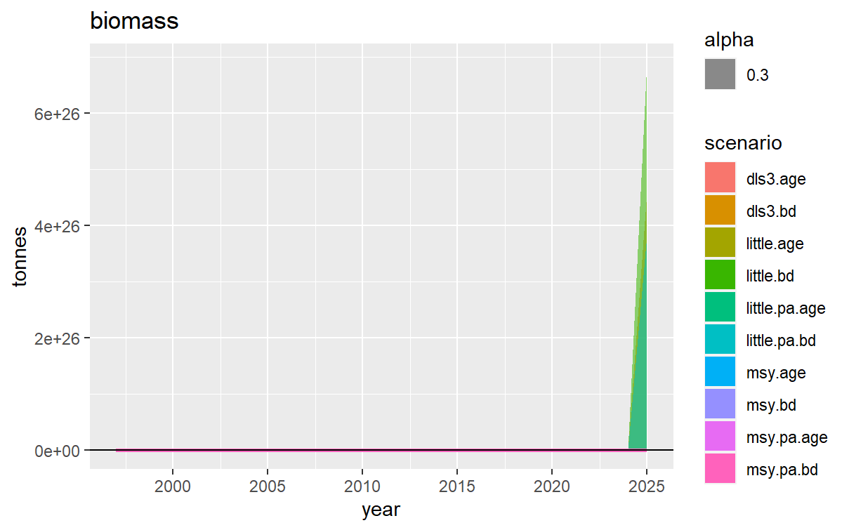
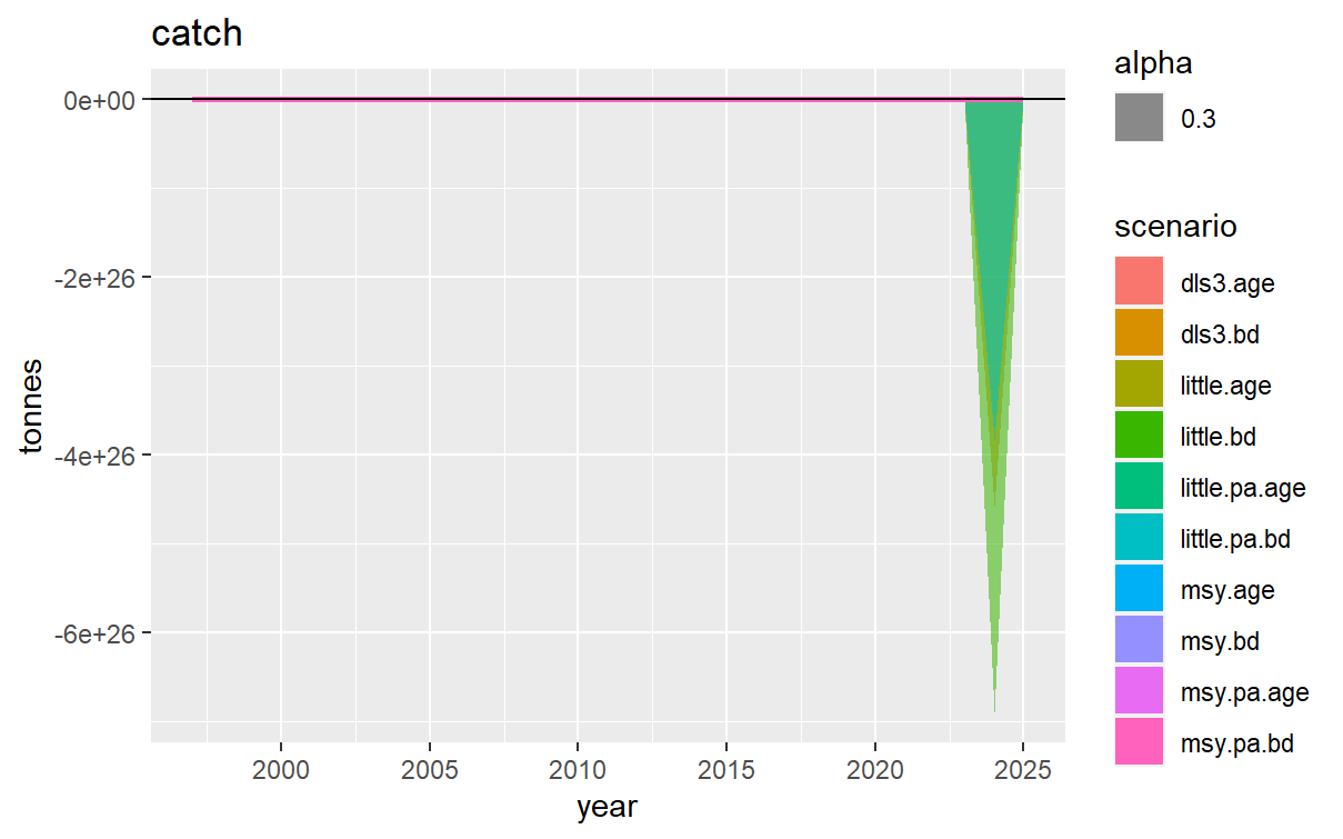
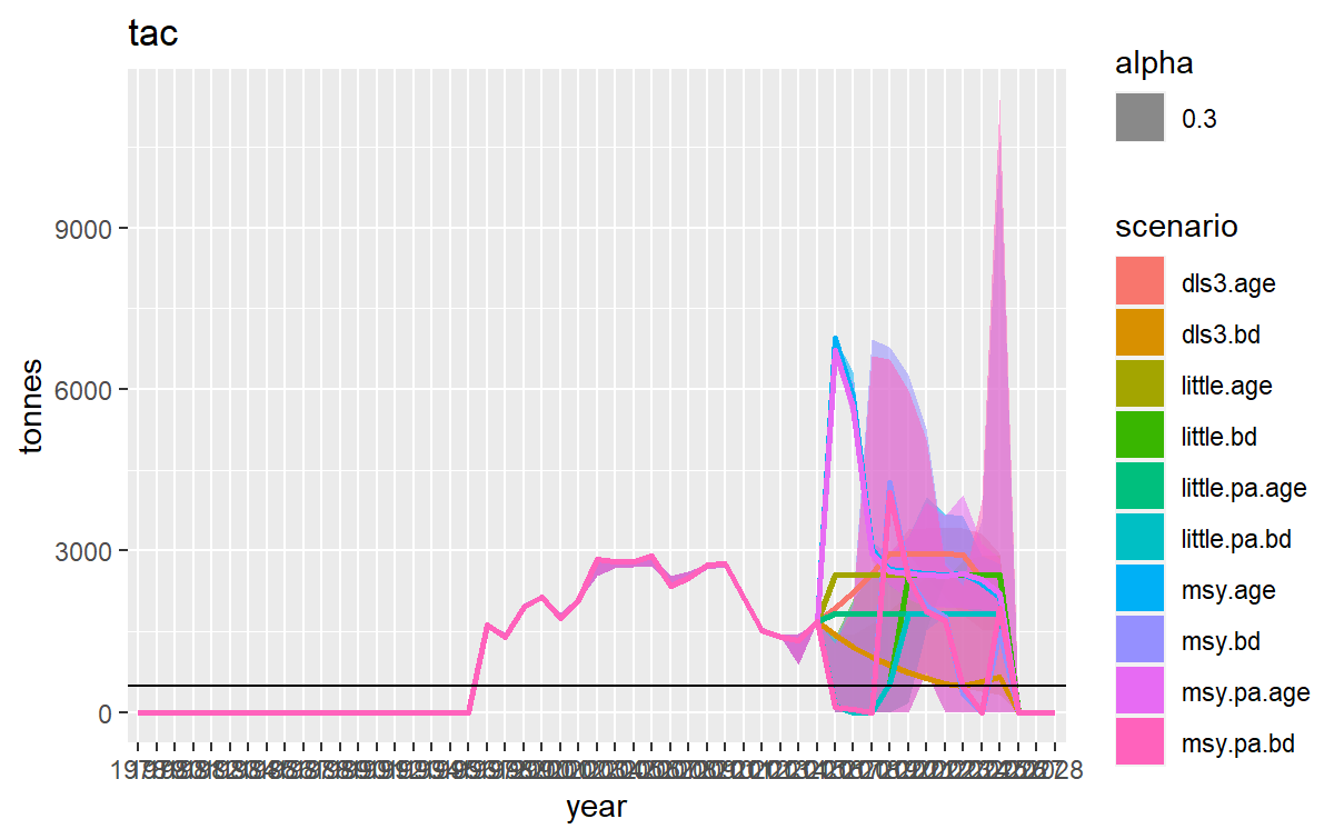
Run FLBEIA in 10 scenarios which differ on:

The structure of the BOM: Age or biomass structured, labeled with ‘age’ or ‘bd’ respectively.
The HCR used:
- The one used by ICES in stocks with absolute estimates of abundance and fishing mortality (scenarios labeled with ‘msy’).
- The one used by ICES for stocks with relative estimates of abundance, survey, CPUE… (scenarios labeled with ‘dls3’).
- A HCR defined y Little et al. in 2011. (scenarios labeled with ‘little’)
The reference points used in the HCR: More or less precautionary reference points. The precautionary scenarios are labeled with ‘pa’.

dls3.bd <- FLBEIA(biols = biols.bd, SRs = NULL, BDs = list(mur = murBD), fleets = fleets.bd, 
                  covars = NULL, indices = list(mur = indices), advice = advice, 
                  main.ctrl, biols.ctrl.bd, fleets.ctrl.bd, covars.ctrl = NULL, 
                  obs.ctrl.ind, assess.ctrl, advice.ctrl.dls3)

############################################################
-                   Year:  38 , Season:  1 
############################################################
************ OPERATING MODEL***************************
------------ BIOLOGICAL OM ------------
-----------------BDPG-----------
------------ FLEETS OM ------------
[1] "~~~~~~~~~~ EFFORT ~~~~~~~~"
[1] "fl"
[1] "~~~~~~ UPDATE CATCH ~~~~~~"
[1] "~~~~~~~~~~ PRICE ~~~~~~~~~~"
[1] "fl"
[1] "****************************** CAPITAL ******************************"
[1] "fl"
------------ COVARS OM ------------
************ MANAGEMENT PROCEDURE ****************************
----------- OBSERVATION MODEL ------------
------------ ASSESSMENT MODEL ------------
----------------- ADVICE -----------------
-----------------  mur  -----------------
############################################################
-                   Year:  39 , Season:  1 
############################################################
************ OPERATING MODEL***************************
------------ BIOLOGICAL OM ------------
-----------------BDPG-----------
------------ FLEETS OM ------------
[1] "~~~~~~~~~~ EFFORT ~~~~~~~~"
[1] "fl"
[1] "~~~~~~ UPDATE CATCH ~~~~~~"
[1] "~~~~~~~~~~ PRICE ~~~~~~~~~~"
[1] "fl"
[1] "****************************** CAPITAL ******************************"
[1] "fl"
------------ COVARS OM ------------
************ MANAGEMENT PROCEDURE ****************************
----------- OBSERVATION MODEL ------------
------------ ASSESSMENT MODEL ------------
----------------- ADVICE -----------------
-----------------  mur  -----------------
############################################################
-                   Year:  40 , Season:  1 
############################################################
************ OPERATING MODEL***************************
------------ BIOLOGICAL OM ------------
-----------------BDPG-----------
------------ FLEETS OM ------------
[1] "~~~~~~~~~~ EFFORT ~~~~~~~~"
[1] "fl"
[1] "~~~~~~ UPDATE CATCH ~~~~~~"
[1] "~~~~~~~~~~ PRICE ~~~~~~~~~~"
[1] "fl"
[1] "****************************** CAPITAL ******************************"
[1] "fl"
------------ COVARS OM ------------
************ MANAGEMENT PROCEDURE ****************************
----------- OBSERVATION MODEL ------------
------------ ASSESSMENT MODEL ------------
----------------- ADVICE -----------------
-----------------  mur  -----------------
############################################################
-                   Year:  41 , Season:  1 
############################################################
************ OPERATING MODEL***************************
------------ BIOLOGICAL OM ------------
-----------------BDPG-----------
------------ FLEETS OM ------------
[1] "~~~~~~~~~~ EFFORT ~~~~~~~~"
[1] "fl"
[1] "~~~~~~ UPDATE CATCH ~~~~~~"
[1] "~~~~~~~~~~ PRICE ~~~~~~~~~~"
[1] "fl"
[1] "****************************** CAPITAL ******************************"
[1] "fl"
------------ COVARS OM ------------
************ MANAGEMENT PROCEDURE ****************************
----------- OBSERVATION MODEL ------------
------------ ASSESSMENT MODEL ------------
----------------- ADVICE -----------------
-----------------  mur  -----------------
############################################################
-                   Year:  42 , Season:  1 
############################################################
************ OPERATING MODEL***************************
------------ BIOLOGICAL OM ------------
-----------------BDPG-----------
------------ FLEETS OM ------------
[1] "~~~~~~~~~~ EFFORT ~~~~~~~~"
[1] "fl"
[1] "~~~~~~ UPDATE CATCH ~~~~~~"
[1] "~~~~~~~~~~ PRICE ~~~~~~~~~~"
[1] "fl"
[1] "****************************** CAPITAL ******************************"
[1] "fl"
------------ COVARS OM ------------
************ MANAGEMENT PROCEDURE ****************************
----------- OBSERVATION MODEL ------------
------------ ASSESSMENT MODEL ------------
----------------- ADVICE -----------------
-----------------  mur  -----------------
############################################################
-                   Year:  43 , Season:  1 
############################################################
************ OPERATING MODEL***************************
------------ BIOLOGICAL OM ------------
-----------------BDPG-----------
------------ FLEETS OM ------------
[1] "~~~~~~~~~~ EFFORT ~~~~~~~~"
[1] "fl"
[1] "~~~~~~ UPDATE CATCH ~~~~~~"
[1] "~~~~~~~~~~ PRICE ~~~~~~~~~~"
[1] "fl"
[1] "****************************** CAPITAL ******************************"
[1] "fl"
------------ COVARS OM ------------
************ MANAGEMENT PROCEDURE ****************************
----------- OBSERVATION MODEL ------------
------------ ASSESSMENT MODEL ------------
----------------- ADVICE -----------------
-----------------  mur  -----------------
############################################################
-                   Year:  44 , Season:  1 
############################################################
************ OPERATING MODEL***************************
------------ BIOLOGICAL OM ------------
-----------------BDPG-----------
------------ FLEETS OM ------------
[1] "~~~~~~~~~~ EFFORT ~~~~~~~~"
[1] "fl"
[1] "~~~~~~ UPDATE CATCH ~~~~~~"
[1] "~~~~~~~~~~ PRICE ~~~~~~~~~~"
[1] "fl"
[1] "****************************** CAPITAL ******************************"
[1] "fl"
------------ COVARS OM ------------
************ MANAGEMENT PROCEDURE ****************************
----------- OBSERVATION MODEL ------------
------------ ASSESSMENT MODEL ------------
----------------- ADVICE -----------------
-----------------  mur  -----------------
############################################################
-                   Year:  45 , Season:  1 
############################################################
************ OPERATING MODEL***************************
------------ BIOLOGICAL OM ------------
-----------------BDPG-----------
------------ FLEETS OM ------------
[1] "~~~~~~~~~~ EFFORT ~~~~~~~~"
[1] "fl"
[1] "~~~~~~ UPDATE CATCH ~~~~~~"
[1] "~~~~~~~~~~ PRICE ~~~~~~~~~~"
[1] "fl"
[1] "****************************** CAPITAL ******************************"
[1] "fl"
------------ COVARS OM ------------
************ MANAGEMENT PROCEDURE ****************************
----------- OBSERVATION MODEL ------------
------------ ASSESSMENT MODEL ------------
----------------- ADVICE -----------------
-----------------  mur  -----------------
############################################################
-                   Year:  46 , Season:  1 
############################################################
************ OPERATING MODEL***************************
------------ BIOLOGICAL OM ------------
-----------------BDPG-----------
------------ FLEETS OM ------------
[1] "~~~~~~~~~~ EFFORT ~~~~~~~~"
[1] "fl"
[1] "~~~~~~ UPDATE CATCH ~~~~~~"
[1] "~~~~~~~~~~ PRICE ~~~~~~~~~~"
[1] "fl"
[1] "****************************** CAPITAL ******************************"
[1] "fl"
------------ COVARS OM ------------
************ MANAGEMENT PROCEDURE ****************************
----------- OBSERVATION MODEL ------------
------------ ASSESSMENT MODEL ------------
----------------- ADVICE -----------------
-----------------  mur  -----------------
############################################################
-                   Year:  47 , Season:  1 
############################################################
************ OPERATING MODEL***************************
------------ BIOLOGICAL OM ------------
-----------------BDPG-----------
------------ FLEETS OM ------------
[1] "~~~~~~~~~~ EFFORT ~~~~~~~~"
[1] "fl"
[1] "~~~~~~ UPDATE CATCH ~~~~~~"
[1] "~~~~~~~~~~ PRICE ~~~~~~~~~~"
[1] "fl"
[1] "****************************** CAPITAL ******************************"
[1] "fl"
------------ COVARS OM ------------
************ MANAGEMENT PROCEDURE ****************************
----------- OBSERVATION MODEL ------------
------------ ASSESSMENT MODEL ------------
----------------- ADVICE -----------------
-----------------  mur  -----------------
############################################################
-                   Year:  48 , Season:  1 
############################################################
************ OPERATING MODEL***************************
------------ BIOLOGICAL OM ------------
-----------------BDPG-----------
------------ FLEETS OM ------------
[1] "~~~~~~~~~~ EFFORT ~~~~~~~~"
[1] "fl"
[1] "~~~~~~ UPDATE CATCH ~~~~~~"
[1] "~~~~~~~~~~ PRICE ~~~~~~~~~~"
[1] "fl"
[1] "****************************** CAPITAL ******************************"
[1] "fl"
------------ COVARS OM ------------

dls3.age <- FLBEIA(biols = biols.age, SRs = list(mur = murSR), BDs = NULL, fleets = fleets.age, 
                   covars = NULL, indices = list(mur = indices), advice = advice, 
                   main.ctrl, biols.ctrl.age, fleets.ctrl.age, covars.ctrl = NULL, 
                   obs.ctrl.ind, assess.ctrl, advice.ctrl.dls3)

############################################################
-                   Year:  38 , Season:  1 
############################################################
************ OPERATING MODEL***************************
------------ BIOLOGICAL OM ------------
-----------------ASPG-----------
------------ FLEETS OM ------------
[1] "~~~~~~~~~~ EFFORT ~~~~~~~~"
[1] "fl"
[1] "~~~~~~ UPDATE CATCH ~~~~~~"
[1] "~~~~~~~~~~ PRICE ~~~~~~~~~~"
[1] "fl"
[1] "****************************** CAPITAL ******************************"
[1] "fl"
------------ COVARS OM ------------
************ MANAGEMENT PROCEDURE ****************************
----------- OBSERVATION MODEL ------------
------------ ASSESSMENT MODEL ------------
----------------- ADVICE -----------------
-----------------  mur  -----------------
############################################################
-                   Year:  39 , Season:  1 
############################################################
************ OPERATING MODEL***************************
------------ BIOLOGICAL OM ------------
-----------------ASPG-----------
------------ FLEETS OM ------------
[1] "~~~~~~~~~~ EFFORT ~~~~~~~~"
[1] "fl"
[1] "~~~~~~ UPDATE CATCH ~~~~~~"
[1] "~~~~~~~~~~ PRICE ~~~~~~~~~~"
[1] "fl"
[1] "****************************** CAPITAL ******************************"
[1] "fl"
------------ COVARS OM ------------
************ MANAGEMENT PROCEDURE ****************************
----------- OBSERVATION MODEL ------------
------------ ASSESSMENT MODEL ------------
----------------- ADVICE -----------------
-----------------  mur  -----------------
############################################################
-                   Year:  40 , Season:  1 
############################################################
************ OPERATING MODEL***************************
------------ BIOLOGICAL OM ------------
-----------------ASPG-----------
------------ FLEETS OM ------------
[1] "~~~~~~~~~~ EFFORT ~~~~~~~~"
[1] "fl"
[1] "~~~~~~ UPDATE CATCH ~~~~~~"
[1] "~~~~~~~~~~ PRICE ~~~~~~~~~~"
[1] "fl"
[1] "****************************** CAPITAL ******************************"
[1] "fl"
------------ COVARS OM ------------
************ MANAGEMENT PROCEDURE ****************************
----------- OBSERVATION MODEL ------------
------------ ASSESSMENT MODEL ------------
----------------- ADVICE -----------------
-----------------  mur  -----------------
############################################################
-                   Year:  41 , Season:  1 
############################################################
************ OPERATING MODEL***************************
------------ BIOLOGICAL OM ------------
-----------------ASPG-----------
------------ FLEETS OM ------------
[1] "~~~~~~~~~~ EFFORT ~~~~~~~~"
[1] "fl"
[1] "~~~~~~ UPDATE CATCH ~~~~~~"
[1] "~~~~~~~~~~ PRICE ~~~~~~~~~~"
[1] "fl"
[1] "****************************** CAPITAL ******************************"
[1] "fl"
------------ COVARS OM ------------
************ MANAGEMENT PROCEDURE ****************************
----------- OBSERVATION MODEL ------------
------------ ASSESSMENT MODEL ------------
----------------- ADVICE -----------------
-----------------  mur  -----------------
############################################################
-                   Year:  42 , Season:  1 
############################################################
************ OPERATING MODEL***************************
------------ BIOLOGICAL OM ------------
-----------------ASPG-----------
------------ FLEETS OM ------------
[1] "~~~~~~~~~~ EFFORT ~~~~~~~~"
[1] "fl"
[1] "~~~~~~ UPDATE CATCH ~~~~~~"
[1] "~~~~~~~~~~ PRICE ~~~~~~~~~~"
[1] "fl"
[1] "****************************** CAPITAL ******************************"
[1] "fl"
------------ COVARS OM ------------
************ MANAGEMENT PROCEDURE ****************************
----------- OBSERVATION MODEL ------------
------------ ASSESSMENT MODEL ------------
----------------- ADVICE -----------------
-----------------  mur  -----------------
############################################################
-                   Year:  43 , Season:  1 
############################################################
************ OPERATING MODEL***************************
------------ BIOLOGICAL OM ------------
-----------------ASPG-----------
------------ FLEETS OM ------------
[1] "~~~~~~~~~~ EFFORT ~~~~~~~~"
[1] "fl"
[1] "~~~~~~ UPDATE CATCH ~~~~~~"
Ba*cth < Ca, for some "a" in stock mur , and iteration  14 
[1] "~~~~~~~~~~ PRICE ~~~~~~~~~~"
[1] "fl"
[1] "****************************** CAPITAL ******************************"
[1] "fl"
------------ COVARS OM ------------
************ MANAGEMENT PROCEDURE ****************************
----------- OBSERVATION MODEL ------------
------------ ASSESSMENT MODEL ------------
----------------- ADVICE -----------------
-----------------  mur  -----------------
############################################################
-                   Year:  44 , Season:  1 
############################################################
************ OPERATING MODEL***************************
------------ BIOLOGICAL OM ------------
-----------------ASPG-----------
------------ FLEETS OM ------------
[1] "~~~~~~~~~~ EFFORT ~~~~~~~~"
[1] "fl"
[1] "~~~~~~ UPDATE CATCH ~~~~~~"
Ba*cth < Ca, for some "a" in stock mur , and iteration  17 
[1] "~~~~~~~~~~ PRICE ~~~~~~~~~~"
[1] "fl"
[1] "****************************** CAPITAL ******************************"
[1] "fl"
------------ COVARS OM ------------
************ MANAGEMENT PROCEDURE ****************************
----------- OBSERVATION MODEL ------------
------------ ASSESSMENT MODEL ------------
----------------- ADVICE -----------------
-----------------  mur  -----------------
############################################################
-                   Year:  45 , Season:  1 
############################################################
************ OPERATING MODEL***************************
------------ BIOLOGICAL OM ------------
-----------------ASPG-----------
------------ FLEETS OM ------------
[1] "~~~~~~~~~~ EFFORT ~~~~~~~~"
[1] "fl"
[1] "~~~~~~ UPDATE CATCH ~~~~~~"
Ba*cth < Ca, for some "a" in stock mur , and iteration  2 
Ba*cth < Ca, for some "a" in stock mur , and iteration  5 
[1] "~~~~~~~~~~ PRICE ~~~~~~~~~~"
[1] "fl"
[1] "****************************** CAPITAL ******************************"
[1] "fl"
------------ COVARS OM ------------
************ MANAGEMENT PROCEDURE ****************************
----------- OBSERVATION MODEL ------------
------------ ASSESSMENT MODEL ------------
----------------- ADVICE -----------------
-----------------  mur  -----------------
############################################################
-                   Year:  46 , Season:  1 
############################################################
************ OPERATING MODEL***************************
------------ BIOLOGICAL OM ------------
-----------------ASPG-----------
------------ FLEETS OM ------------
[1] "~~~~~~~~~~ EFFORT ~~~~~~~~"
[1] "fl"
[1] "~~~~~~ UPDATE CATCH ~~~~~~"
[1] "~~~~~~~~~~ PRICE ~~~~~~~~~~"
[1] "fl"
[1] "****************************** CAPITAL ******************************"
[1] "fl"
------------ COVARS OM ------------
************ MANAGEMENT PROCEDURE ****************************
----------- OBSERVATION MODEL ------------
------------ ASSESSMENT MODEL ------------
----------------- ADVICE -----------------
-----------------  mur  -----------------
############################################################
-                   Year:  47 , Season:  1 
############################################################
************ OPERATING MODEL***************************
------------ BIOLOGICAL OM ------------
-----------------ASPG-----------
------------ FLEETS OM ------------
[1] "~~~~~~~~~~ EFFORT ~~~~~~~~"
[1] "fl"
[1] "~~~~~~ UPDATE CATCH ~~~~~~"
Ba*cth < Ca, for some "a" in stock mur , and iteration  8 
Ba*cth < Ca, for some "a" in stock mur , and iteration  13 
[1] "~~~~~~~~~~ PRICE ~~~~~~~~~~"
[1] "fl"
[1] "****************************** CAPITAL ******************************"
[1] "fl"
------------ COVARS OM ------------
************ MANAGEMENT PROCEDURE ****************************
----------- OBSERVATION MODEL ------------
------------ ASSESSMENT MODEL ------------
----------------- ADVICE -----------------
-----------------  mur  -----------------
############################################################
-                   Year:  48 , Season:  1 
############################################################
************ OPERATING MODEL***************************
------------ BIOLOGICAL OM ------------
-----------------ASPG-----------
------------ FLEETS OM ------------
[1] "~~~~~~~~~~ EFFORT ~~~~~~~~"
[1] "fl"
[1] "~~~~~~ UPDATE CATCH ~~~~~~"
Ba*cth < Ca, for some "a" in stock mur , and iteration  7 
Ba*cth < Ca, for some "a" in stock mur , and iteration  13 
[1] "~~~~~~~~~~ PRICE ~~~~~~~~~~"
[1] "fl"
[1] "****************************** CAPITAL ******************************"
[1] "fl"
------------ COVARS OM ------------

#main.ctrl[[1]][2] <- 2022

little.bd <- FLBEIA(biols = biols.bd, SRs = NULL, BDs = list(mur = murBD), fleets = fleets.bd, 
                    covars = NULL, indices = list(mur = indices), advice = advice, 
                    main.ctrl, biols.ctrl.bd, fleets.ctrl.bd, covars.ctrl = NULL, 
                    obs.ctrl.ind, assess.ctrl, advice.ctrl.little)

############################################################
-                   Year:  38 , Season:  1 
############################################################
************ OPERATING MODEL***************************
------------ BIOLOGICAL OM ------------
-----------------BDPG-----------
------------ FLEETS OM ------------
[1] "~~~~~~~~~~ EFFORT ~~~~~~~~"
[1] "fl"
[1] "~~~~~~ UPDATE CATCH ~~~~~~"
[1] "~~~~~~~~~~ PRICE ~~~~~~~~~~"
[1] "fl"
[1] "****************************** CAPITAL ******************************"
[1] "fl"
------------ COVARS OM ------------
************ MANAGEMENT PROCEDURE ****************************
----------- OBSERVATION MODEL ------------
------------ ASSESSMENT MODEL ------------
----------------- ADVICE -----------------
-----------------  mur  -----------------
.......... 77.28675 724.5449 0 0 119.4003 0 390.1174 488.1391 360.7495 0 396.1847 0 0 140.5866 663.8009 1330.889 2555.781 65.98356 1063.897 0 ............
############################################################
-                   Year:  39 , Season:  1 
############################################################
************ OPERATING MODEL***************************
------------ BIOLOGICAL OM ------------
-----------------BDPG-----------
------------ FLEETS OM ------------
[1] "~~~~~~~~~~ EFFORT ~~~~~~~~"
[1] "fl"
[1] "~~~~~~ UPDATE CATCH ~~~~~~"
[1] "~~~~~~~~~~ PRICE ~~~~~~~~~~"
[1] "fl"
[1] "****************************** CAPITAL ******************************"
[1] "fl"
------------ COVARS OM ------------
************ MANAGEMENT PROCEDURE ****************************
----------- OBSERVATION MODEL ------------
------------ ASSESSMENT MODEL ------------
----------------- ADVICE -----------------
-----------------  mur  -----------------
.......... 0 1939.297 0 0 0 0 558.8939 1005.683 368.9112 0 474.5182 0 0 3.738719 990.5581 2085.506 2555.781 0 1951.016 0 ............
############################################################
-                   Year:  40 , Season:  1 
############################################################
************ OPERATING MODEL***************************
------------ BIOLOGICAL OM ------------
-----------------BDPG-----------
------------ FLEETS OM ------------
[1] "~~~~~~~~~~ EFFORT ~~~~~~~~"
[1] "fl"
[1] "~~~~~~ UPDATE CATCH ~~~~~~"
[1] "~~~~~~~~~~ PRICE ~~~~~~~~~~"
[1] "fl"
[1] "****************************** CAPITAL ******************************"
[1] "fl"
------------ COVARS OM ------------
************ MANAGEMENT PROCEDURE ****************************
----------- OBSERVATION MODEL ------------
------------ ASSESSMENT MODEL ------------
----------------- ADVICE -----------------
-----------------  mur  -----------------
.......... 0 2555.781 0 0 0 0 1024.713 2555.781 467.5488 0 1364.411 0 0 0 1786.259 2555.781 2555.781 0 2555.781 0 ............
############################################################
-                   Year:  41 , Season:  1 
############################################################
************ OPERATING MODEL***************************
------------ BIOLOGICAL OM ------------
-----------------BDPG-----------
------------ FLEETS OM ------------
[1] "~~~~~~~~~~ EFFORT ~~~~~~~~"
[1] "fl"
[1] "~~~~~~ UPDATE CATCH ~~~~~~"
[1] "~~~~~~~~~~ PRICE ~~~~~~~~~~"
[1] "fl"
[1] "****************************** CAPITAL ******************************"
[1] "fl"
------------ COVARS OM ------------
************ MANAGEMENT PROCEDURE ****************************
----------- OBSERVATION MODEL ------------
------------ ASSESSMENT MODEL ------------
----------------- ADVICE -----------------
-----------------  mur  -----------------
.......... 251.1761 2555.781 260.0679 0 0 0 2555.781 2555.781 1238.808 0 2555.781 0 0 308.2786 2555.781 2555.781 2555.781 774.2501 2555.781 0 ............
############################################################
-                   Year:  42 , Season:  1 
############################################################
************ OPERATING MODEL***************************
------------ BIOLOGICAL OM ------------
-----------------BDPG-----------
------------ FLEETS OM ------------
[1] "~~~~~~~~~~ EFFORT ~~~~~~~~"
[1] "fl"
[1] "~~~~~~ UPDATE CATCH ~~~~~~"
[1] "~~~~~~~~~~ PRICE ~~~~~~~~~~"
[1] "fl"
[1] "****************************** CAPITAL ******************************"
[1] "fl"
------------ COVARS OM ------------
************ MANAGEMENT PROCEDURE ****************************
----------- OBSERVATION MODEL ------------
------------ ASSESSMENT MODEL ------------
----------------- ADVICE -----------------
-----------------  mur  -----------------
.......... 2171.474 2555.781 2555.781 214.0704 198.7346 300.0314 2555.781 2555.781 2555.781 428.9168 2555.781 330.3201 0 1010.933 2555.781 2555.781 2555.781 2555.781 2555.781 232.6673 ............
############################################################
-                   Year:  43 , Season:  1 
############################################################
************ OPERATING MODEL***************************
------------ BIOLOGICAL OM ------------
-----------------BDPG-----------
------------ FLEETS OM ------------
[1] "~~~~~~~~~~ EFFORT ~~~~~~~~"
[1] "fl"
[1] "~~~~~~ UPDATE CATCH ~~~~~~"
[1] "~~~~~~~~~~ PRICE ~~~~~~~~~~"
[1] "fl"
[1] "****************************** CAPITAL ******************************"
[1] "fl"
------------ COVARS OM ------------
************ MANAGEMENT PROCEDURE ****************************
----------- OBSERVATION MODEL ------------
------------ ASSESSMENT MODEL ------------
----------------- ADVICE -----------------
-----------------  mur  -----------------
.......... 2555.781 2555.781 2555.781 1876.688 1600.599 2217.479 2555.781 2555.781 2555.781 2051.561 2555.781 2208.62 3.251452 2555.781 2555.781 2555.781 2555.781 2555.781 2555.781 2231.502 ............
############################################################
-                   Year:  44 , Season:  1 
############################################################
************ OPERATING MODEL***************************
------------ BIOLOGICAL OM ------------
-----------------BDPG-----------
------------ FLEETS OM ------------
[1] "~~~~~~~~~~ EFFORT ~~~~~~~~"
[1] "fl"
[1] "~~~~~~ UPDATE CATCH ~~~~~~"
[1] "~~~~~~~~~~ PRICE ~~~~~~~~~~"
[1] "fl"
[1] "****************************** CAPITAL ******************************"
[1] "fl"
------------ COVARS OM ------------
************ MANAGEMENT PROCEDURE ****************************
----------- OBSERVATION MODEL ------------
------------ ASSESSMENT MODEL ------------
----------------- ADVICE -----------------
-----------------  mur  -----------------
.......... 2555.781 2555.781 2555.781 2555.781 2555.781 2555.781 2555.781 2555.781 2555.781 2555.781 2555.781 2555.781 1051.45 2555.781 2555.781 2555.781 2555.781 2555.781 2555.781 2555.781 ............
############################################################
-                   Year:  45 , Season:  1 
############################################################
************ OPERATING MODEL***************************
------------ BIOLOGICAL OM ------------
-----------------BDPG-----------
------------ FLEETS OM ------------
[1] "~~~~~~~~~~ EFFORT ~~~~~~~~"
[1] "fl"
[1] "~~~~~~ UPDATE CATCH ~~~~~~"
[1] "~~~~~~~~~~ PRICE ~~~~~~~~~~"
[1] "fl"
[1] "****************************** CAPITAL ******************************"
[1] "fl"
------------ COVARS OM ------------
************ MANAGEMENT PROCEDURE ****************************
----------- OBSERVATION MODEL ------------
------------ ASSESSMENT MODEL ------------
----------------- ADVICE -----------------
-----------------  mur  -----------------
.......... 2555.781 2555.781 2555.781 2555.781 2555.781 2555.781 2555.781 2555.781 2555.781 2555.781 2555.781 2555.781 2555.781 2555.781 2555.781 2555.781 2555.781 2555.781 2555.781 2555.781 ............
############################################################
-                   Year:  46 , Season:  1 
############################################################
************ OPERATING MODEL***************************
------------ BIOLOGICAL OM ------------
-----------------BDPG-----------
------------ FLEETS OM ------------
[1] "~~~~~~~~~~ EFFORT ~~~~~~~~"
[1] "fl"
[1] "~~~~~~ UPDATE CATCH ~~~~~~"
[1] "~~~~~~~~~~ PRICE ~~~~~~~~~~"
[1] "fl"
[1] "****************************** CAPITAL ******************************"
[1] "fl"
------------ COVARS OM ------------
************ MANAGEMENT PROCEDURE ****************************
----------- OBSERVATION MODEL ------------
------------ ASSESSMENT MODEL ------------
----------------- ADVICE -----------------
-----------------  mur  -----------------
.......... 2555.781 2555.781 2555.781 2555.781 2555.781 2555.781 2478.845 2281.784 2555.781 2555.781 2555.781 2555.781 2555.781 2555.781 2555.781 2555.781 2555.781 2555.781 2555.781 2555.781 ............
############################################################
-                   Year:  47 , Season:  1 
############################################################
************ OPERATING MODEL***************************
------------ BIOLOGICAL OM ------------
-----------------BDPG-----------
------------ FLEETS OM ------------
[1] "~~~~~~~~~~ EFFORT ~~~~~~~~"
[1] "fl"
[1] "~~~~~~ UPDATE CATCH ~~~~~~"
[1] "~~~~~~~~~~ PRICE ~~~~~~~~~~"
[1] "fl"
[1] "****************************** CAPITAL ******************************"
[1] "fl"
------------ COVARS OM ------------
************ MANAGEMENT PROCEDURE ****************************
----------- OBSERVATION MODEL ------------
------------ ASSESSMENT MODEL ------------
----------------- ADVICE -----------------
-----------------  mur  -----------------
.......... 2555.781 2555.781 2555.781 2555.781 2555.781 2555.781 2404.228 1380.08 2555.781 2555.781 2555.781 2555.781 2555.781 2555.781 2555.781 2555.781 2555.781 2555.781 2555.781 2555.781 ............
############################################################
-                   Year:  48 , Season:  1 
############################################################
************ OPERATING MODEL***************************
------------ BIOLOGICAL OM ------------
-----------------BDPG-----------
------------ FLEETS OM ------------
[1] "~~~~~~~~~~ EFFORT ~~~~~~~~"
[1] "fl"
[1] "~~~~~~ UPDATE CATCH ~~~~~~"
[1] "~~~~~~~~~~ PRICE ~~~~~~~~~~"
[1] "fl"
[1] "****************************** CAPITAL ******************************"
[1] "fl"
------------ COVARS OM ------------

little.age <- FLBEIA(biols = biols.age, SRs = list(mur = murSR), BDs = NULL, fleets = fleets.age, 
                     covars = NULL, indices = list(mur = indices), advice = advice, 
                     main.ctrl, biols.ctrl.age, fleets.ctrl.age, covars.ctrl = NULL, 
                     obs.ctrl.ind, assess.ctrl, advice.ctrl.little)

############################################################
-                   Year:  38 , Season:  1 
############################################################
************ OPERATING MODEL***************************
------------ BIOLOGICAL OM ------------
-----------------ASPG-----------
------------ FLEETS OM ------------
[1] "~~~~~~~~~~ EFFORT ~~~~~~~~"
[1] "fl"
[1] "~~~~~~ UPDATE CATCH ~~~~~~"
[1] "~~~~~~~~~~ PRICE ~~~~~~~~~~"
[1] "fl"
[1] "****************************** CAPITAL ******************************"
[1] "fl"
------------ COVARS OM ------------
************ MANAGEMENT PROCEDURE ****************************
----------- OBSERVATION MODEL ------------
------------ ASSESSMENT MODEL ------------
----------------- ADVICE -----------------
-----------------  mur  -----------------
.......... 2555.781 2555.781 2555.781 2555.781 2555.781 2555.781 2555.781 2555.781 2555.781 2555.781 2555.781 2555.781 2555.781 2555.781 2555.781 2555.781 2555.781 2555.781 2555.781 2555.781 ............
############################################################
-                   Year:  39 , Season:  1 
############################################################
************ OPERATING MODEL***************************
------------ BIOLOGICAL OM ------------
-----------------ASPG-----------
------------ FLEETS OM ------------
[1] "~~~~~~~~~~ EFFORT ~~~~~~~~"
[1] "fl"
[1] "~~~~~~ UPDATE CATCH ~~~~~~"
[1] "~~~~~~~~~~ PRICE ~~~~~~~~~~"
[1] "fl"
[1] "****************************** CAPITAL ******************************"
[1] "fl"
------------ COVARS OM ------------
************ MANAGEMENT PROCEDURE ****************************
----------- OBSERVATION MODEL ------------
------------ ASSESSMENT MODEL ------------
----------------- ADVICE -----------------
-----------------  mur  -----------------
.......... 2555.781 2555.781 2555.781 2555.781 2555.781 2555.781 2555.781 2555.781 2555.781 2555.781 2555.781 2555.781 2555.781 2555.781 2555.781 2555.781 2555.781 2555.781 2555.781 2555.781 ............
############################################################
-                   Year:  40 , Season:  1 
############################################################
************ OPERATING MODEL***************************
------------ BIOLOGICAL OM ------------
-----------------ASPG-----------
------------ FLEETS OM ------------
[1] "~~~~~~~~~~ EFFORT ~~~~~~~~"
[1] "fl"
[1] "~~~~~~ UPDATE CATCH ~~~~~~"
[1] "~~~~~~~~~~ PRICE ~~~~~~~~~~"
[1] "fl"
[1] "****************************** CAPITAL ******************************"
[1] "fl"
------------ COVARS OM ------------
************ MANAGEMENT PROCEDURE ****************************
----------- OBSERVATION MODEL ------------
------------ ASSESSMENT MODEL ------------
----------------- ADVICE -----------------
-----------------  mur  -----------------
.......... 2555.781 2555.781 2555.781 2555.781 2555.781 2555.781 2555.781 2555.781 2555.781 2555.781 2555.781 2555.781 2555.781 2555.781 2555.781 2555.781 2555.781 2555.781 2555.781 2555.781 ............
############################################################
-                   Year:  41 , Season:  1 
############################################################
************ OPERATING MODEL***************************
------------ BIOLOGICAL OM ------------
-----------------ASPG-----------
------------ FLEETS OM ------------
[1] "~~~~~~~~~~ EFFORT ~~~~~~~~"
[1] "fl"
[1] "~~~~~~ UPDATE CATCH ~~~~~~"
[1] "~~~~~~~~~~ PRICE ~~~~~~~~~~"
[1] "fl"
[1] "****************************** CAPITAL ******************************"
[1] "fl"
------------ COVARS OM ------------
************ MANAGEMENT PROCEDURE ****************************
----------- OBSERVATION MODEL ------------
------------ ASSESSMENT MODEL ------------
----------------- ADVICE -----------------
-----------------  mur  -----------------
.......... 2555.781 2555.781 2555.781 2555.781 2555.781 2555.781 2555.781 2555.781 2555.781 2555.781 2555.781 2555.781 2555.781 2555.781 2555.781 2555.781 2555.781 2555.781 2555.781 2555.781 ............
############################################################
-                   Year:  42 , Season:  1 
############################################################
************ OPERATING MODEL***************************
------------ BIOLOGICAL OM ------------
-----------------ASPG-----------
------------ FLEETS OM ------------
[1] "~~~~~~~~~~ EFFORT ~~~~~~~~"
[1] "fl"
[1] "~~~~~~ UPDATE CATCH ~~~~~~"
Ba*cth < Ca, for some "a" in stock mur , and iteration  14 
[1] "~~~~~~~~~~ PRICE ~~~~~~~~~~"
[1] "fl"
[1] "****************************** CAPITAL ******************************"
[1] "fl"
------------ COVARS OM ------------
************ MANAGEMENT PROCEDURE ****************************
----------- OBSERVATION MODEL ------------
------------ ASSESSMENT MODEL ------------
----------------- ADVICE -----------------
-----------------  mur  -----------------
.......... 2555.781 2555.781 2555.781 2555.781 2555.781 2555.781 2555.781 2555.781 2555.781 2555.781 2555.781 2555.781 2555.781 2555.781 2555.781 2555.781 2555.781 2555.781 2555.781 2555.781 ............
############################################################
-                   Year:  43 , Season:  1 
############################################################
************ OPERATING MODEL***************************
------------ BIOLOGICAL OM ------------
-----------------ASPG-----------
------------ FLEETS OM ------------
[1] "~~~~~~~~~~ EFFORT ~~~~~~~~"
[1] "fl"
[1] "~~~~~~ UPDATE CATCH ~~~~~~"
[1] "~~~~~~~~~~ PRICE ~~~~~~~~~~"
[1] "fl"
[1] "****************************** CAPITAL ******************************"
[1] "fl"
------------ COVARS OM ------------
************ MANAGEMENT PROCEDURE ****************************
----------- OBSERVATION MODEL ------------
------------ ASSESSMENT MODEL ------------
----------------- ADVICE -----------------
-----------------  mur  -----------------
.......... 2555.781 2555.781 2555.781 2555.781 2555.781 2555.781 2555.781 2555.781 2555.781 2555.781 2555.781 2555.781 2555.781 2555.781 2555.781 2555.781 2555.781 2555.781 2555.781 2555.781 ............
############################################################
-                   Year:  44 , Season:  1 
############################################################
************ OPERATING MODEL***************************
------------ BIOLOGICAL OM ------------
-----------------ASPG-----------
------------ FLEETS OM ------------
[1] "~~~~~~~~~~ EFFORT ~~~~~~~~"
[1] "fl"
[1] "~~~~~~ UPDATE CATCH ~~~~~~"
Ba*cth < Ca, for some "a" in stock mur , and iteration  20 
[1] "~~~~~~~~~~ PRICE ~~~~~~~~~~"
[1] "fl"
[1] "****************************** CAPITAL ******************************"
[1] "fl"
------------ COVARS OM ------------
************ MANAGEMENT PROCEDURE ****************************
----------- OBSERVATION MODEL ------------
------------ ASSESSMENT MODEL ------------
----------------- ADVICE -----------------
-----------------  mur  -----------------
.......... 2555.781 2555.781 2555.781 2555.781 2555.781 2555.781 2555.781 2555.781 2555.781 2555.781 2555.781 2555.781 2555.781 2555.781 2555.781 2555.781 2555.781 2555.781 2555.781 2555.781 ............
############################################################
-                   Year:  45 , Season:  1 
############################################################
************ OPERATING MODEL***************************
------------ BIOLOGICAL OM ------------
-----------------ASPG-----------
------------ FLEETS OM ------------
[1] "~~~~~~~~~~ EFFORT ~~~~~~~~"
[1] "fl"
[1] "~~~~~~ UPDATE CATCH ~~~~~~"
Ba*cth < Ca, for some "a" in stock mur , and iteration  2 
Ba*cth < Ca, for some "a" in stock mur , and iteration  12 
Ba*cth < Ca, for some "a" in stock mur , and iteration  20 
[1] "~~~~~~~~~~ PRICE ~~~~~~~~~~"
[1] "fl"
[1] "****************************** CAPITAL ******************************"
[1] "fl"
------------ COVARS OM ------------
************ MANAGEMENT PROCEDURE ****************************
----------- OBSERVATION MODEL ------------
------------ ASSESSMENT MODEL ------------
----------------- ADVICE -----------------
-----------------  mur  -----------------
.......... 2555.781 2555.781 2555.781 2555.781 2555.781 2555.781 2555.781 2555.781 2555.781 2555.781 2555.781 2555.781 2555.781 2555.781 2555.781 2555.781 2555.781 2555.781 2555.781 2555.781 ............
############################################################
-                   Year:  46 , Season:  1 
############################################################
************ OPERATING MODEL***************************
------------ BIOLOGICAL OM ------------
-----------------ASPG-----------
------------ FLEETS OM ------------
[1] "~~~~~~~~~~ EFFORT ~~~~~~~~"
[1] "fl"
[1] "~~~~~~ UPDATE CATCH ~~~~~~"
[1] "~~~~~~~~~~ PRICE ~~~~~~~~~~"
[1] "fl"
[1] "****************************** CAPITAL ******************************"
[1] "fl"
------------ COVARS OM ------------
************ MANAGEMENT PROCEDURE ****************************
----------- OBSERVATION MODEL ------------
------------ ASSESSMENT MODEL ------------
----------------- ADVICE -----------------
-----------------  mur  -----------------
.......... 2555.781 2555.781 2555.781 2555.781 2555.781 2555.781 2555.781 2555.781 2555.781 2555.781 2555.781 2555.781 2555.781 2555.781 2555.781 2555.781 2555.781 2555.781 2555.781 2555.781 ............
############################################################
-                   Year:  47 , Season:  1 
############################################################
************ OPERATING MODEL***************************
------------ BIOLOGICAL OM ------------
-----------------ASPG-----------
------------ FLEETS OM ------------
[1] "~~~~~~~~~~ EFFORT ~~~~~~~~"
[1] "fl"
[1] "~~~~~~ UPDATE CATCH ~~~~~~"
Ba*cth < Ca, for some "a" in stock mur , and iteration  2 
[1] "~~~~~~~~~~ PRICE ~~~~~~~~~~"
[1] "fl"
[1] "****************************** CAPITAL ******************************"
[1] "fl"
------------ COVARS OM ------------
************ MANAGEMENT PROCEDURE ****************************
----------- OBSERVATION MODEL ------------
------------ ASSESSMENT MODEL ------------
----------------- ADVICE -----------------
-----------------  mur  -----------------
.......... 2555.781 2555.781 2555.781 2555.781 2555.781 2555.781 2555.781 2555.781 2555.781 2555.781 2555.781 2555.781 2555.781 2555.781 2555.781 2555.781 2555.781 2555.781 2555.781 2555.781 ............
############################################################
-                   Year:  48 , Season:  1 
############################################################
************ OPERATING MODEL***************************
------------ BIOLOGICAL OM ------------
-----------------ASPG-----------
------------ FLEETS OM ------------
[1] "~~~~~~~~~~ EFFORT ~~~~~~~~"
[1] "fl"
[1] "~~~~~~ UPDATE CATCH ~~~~~~"
[1] "~~~~~~~~~~ PRICE ~~~~~~~~~~"
[1] "fl"
[1] "****************************** CAPITAL ******************************"
[1] "fl"
------------ COVARS OM ------------

biols.bd[[1]]@range[1:3] <- NA
msy.bd <- FLBEIA(biols = biols.bd, SRs = NULL, BDs = list(mur = murBD), fleets = fleets.bd, 
                 covars = NULL, indices = NULL, advice = advice, main.ctrl, 
                 biols.ctrl.bd, fleets.ctrl.bd, covars.ctrl = NULL, 
                 obs.ctrl.stk, assess.ctrl, advice.ctrl.msy)

############################################################
-                   Year:  38 , Season:  1 
############################################################
************ OPERATING MODEL***************************
------------ BIOLOGICAL OM ------------
-----------------BDPG-----------
------------ FLEETS OM ------------
[1] "~~~~~~~~~~ EFFORT ~~~~~~~~"
[1] "fl"
[1] "~~~~~~ UPDATE CATCH ~~~~~~"
[1] "~~~~~~~~~~ PRICE ~~~~~~~~~~"
[1] "fl"
[1] "****************************** CAPITAL ******************************"
[1] "fl"
------------ COVARS OM ------------
************ MANAGEMENT PROCEDURE ****************************
----------- OBSERVATION MODEL ------------
------------ ASSESSMENT MODEL ------------
----------------- ADVICE -----------------
-----------------  mur  -----------------
 [1] 0.8777591 0.8346375 0.0000000 0.7984378 1.0462008 0.0000000 1.0462008
 [8] 0.9817660 1.0462008 0.0000000 1.0036610 0.8223011 0.9339261 0.8157589
[15] 1.0462008 1.0462008 1.0462008 0.9173131 0.7911501 0.0000000
############################################################
-                   Year:  39 , Season:  1 
############################################################
************ OPERATING MODEL***************************
------------ BIOLOGICAL OM ------------
-----------------BDPG-----------
------------ FLEETS OM ------------
[1] "~~~~~~~~~~ EFFORT ~~~~~~~~"
[1] "fl"
[1] "~~~~~~ UPDATE CATCH ~~~~~~"
[1] "~~~~~~~~~~ PRICE ~~~~~~~~~~"
[1] "fl"
[1] "****************************** CAPITAL ******************************"
[1] "fl"
------------ COVARS OM ------------
************ MANAGEMENT PROCEDURE ****************************
----------- OBSERVATION MODEL ------------
------------ ASSESSMENT MODEL ------------
----------------- ADVICE -----------------
-----------------  mur  -----------------
 [1] 0.8307532 1.0462008 0.0000000 0.0000000 1.0316473 0.0000000 1.0462008
 [8] 1.0462008 1.0462008 0.0000000 1.0462008 0.0000000 0.0000000 0.0000000
[15] 1.0462008 1.0462008 1.0462008 0.8944886 1.0462008 0.0000000
############################################################
-                   Year:  40 , Season:  1 
############################################################
************ OPERATING MODEL***************************
------------ BIOLOGICAL OM ------------
-----------------BDPG-----------
------------ FLEETS OM ------------
[1] "~~~~~~~~~~ EFFORT ~~~~~~~~"
[1] "fl"
[1] "~~~~~~ UPDATE CATCH ~~~~~~"
[1] "~~~~~~~~~~ PRICE ~~~~~~~~~~"
[1] "fl"
[1] "****************************** CAPITAL ******************************"
[1] "fl"
------------ COVARS OM ------------
************ MANAGEMENT PROCEDURE ****************************
----------- OBSERVATION MODEL ------------
------------ ASSESSMENT MODEL ------------
----------------- ADVICE -----------------
-----------------  mur  -----------------
 [1] 0.000000 1.046201 0.000000 0.000000 0.000000 0.000000 1.046201 1.046201
 [9] 1.046201 0.000000 1.046201 0.000000 0.000000 0.000000 1.046201 1.046201
[17] 1.046201 0.000000 1.046201 0.000000
############################################################
-                   Year:  41 , Season:  1 
############################################################
************ OPERATING MODEL***************************
------------ BIOLOGICAL OM ------------
-----------------BDPG-----------
------------ FLEETS OM ------------
[1] "~~~~~~~~~~ EFFORT ~~~~~~~~"
[1] "fl"
[1] "~~~~~~ UPDATE CATCH ~~~~~~"
[1] "~~~~~~~~~~ PRICE ~~~~~~~~~~"
[1] "fl"
[1] "****************************** CAPITAL ******************************"
[1] "fl"
------------ COVARS OM ------------
************ MANAGEMENT PROCEDURE ****************************
----------- OBSERVATION MODEL ------------
------------ ASSESSMENT MODEL ------------
----------------- ADVICE -----------------
-----------------  mur  -----------------
 [1] 1.046201 1.046201 1.046201 0.000000 0.000000 1.046201 1.046201 1.046201
 [9] 1.046201 1.046201 1.046201 0.000000 0.000000 1.046201 1.046201 1.046201
[17] 1.046201 1.046201 1.046201 0.000000
############################################################
-                   Year:  42 , Season:  1 
############################################################
************ OPERATING MODEL***************************
------------ BIOLOGICAL OM ------------
-----------------BDPG-----------
------------ FLEETS OM ------------
[1] "~~~~~~~~~~ EFFORT ~~~~~~~~"
[1] "fl"
[1] "~~~~~~ UPDATE CATCH ~~~~~~"
[1] "~~~~~~~~~~ PRICE ~~~~~~~~~~"
[1] "fl"
[1] "****************************** CAPITAL ******************************"
[1] "fl"
------------ COVARS OM ------------
************ MANAGEMENT PROCEDURE ****************************
----------- OBSERVATION MODEL ------------
------------ ASSESSMENT MODEL ------------
----------------- ADVICE -----------------
-----------------  mur  -----------------
 [1] 1.046201 1.046201 1.046201 1.046201 0.000000 1.046201 1.046201 1.046201
 [9] 1.046201 1.046201 1.046201 1.046201 0.000000 1.046201 1.046201 1.046201
[17] 1.046201 1.046201 1.046201 1.046201
############################################################
-                   Year:  43 , Season:  1 
############################################################
************ OPERATING MODEL***************************
------------ BIOLOGICAL OM ------------
-----------------BDPG-----------
------------ FLEETS OM ------------
[1] "~~~~~~~~~~ EFFORT ~~~~~~~~"
[1] "fl"
[1] "~~~~~~ UPDATE CATCH ~~~~~~"
[1] "~~~~~~~~~~ PRICE ~~~~~~~~~~"
[1] "fl"
[1] "****************************** CAPITAL ******************************"
[1] "fl"
------------ COVARS OM ------------
************ MANAGEMENT PROCEDURE ****************************
----------- OBSERVATION MODEL ------------
------------ ASSESSMENT MODEL ------------
----------------- ADVICE -----------------
-----------------  mur  -----------------
 [1] 1.0462008 1.0462008 1.0462008 1.0462008 1.0141843 1.0462008 1.0462008
 [8] 0.9414571 1.0462008 1.0462008 1.0462008 1.0462008 0.0000000 1.0462008
[15] 1.0462008 1.0462008 1.0462008 1.0462008 0.9596531 1.0462008
############################################################
-                   Year:  44 , Season:  1 
############################################################
************ OPERATING MODEL***************************
------------ BIOLOGICAL OM ------------
-----------------BDPG-----------
------------ FLEETS OM ------------
[1] "~~~~~~~~~~ EFFORT ~~~~~~~~"
[1] "fl"
[1] "~~~~~~ UPDATE CATCH ~~~~~~"
[1] "~~~~~~~~~~ PRICE ~~~~~~~~~~"
[1] "fl"
[1] "****************************** CAPITAL ******************************"
[1] "fl"
------------ COVARS OM ------------
************ MANAGEMENT PROCEDURE ****************************
----------- OBSERVATION MODEL ------------
------------ ASSESSMENT MODEL ------------
----------------- ADVICE -----------------
-----------------  mur  -----------------
 [1] 1.0462008 0.0000000 1.0462008 1.0462008 1.0462008 1.0462008 1.0033669
 [8] 0.0000000 0.8948305 1.0462008 0.0000000 1.0462008 0.8194336 1.0462008
[15] 1.0462008 1.0462008 1.0462008 1.0462008 0.0000000 1.0462008
############################################################
-                   Year:  45 , Season:  1 
############################################################
************ OPERATING MODEL***************************
------------ BIOLOGICAL OM ------------
-----------------BDPG-----------
------------ FLEETS OM ------------
[1] "~~~~~~~~~~ EFFORT ~~~~~~~~"
[1] "fl"
[1] "~~~~~~ UPDATE CATCH ~~~~~~"
[1] "~~~~~~~~~~ PRICE ~~~~~~~~~~"
[1] "fl"
[1] "****************************** CAPITAL ******************************"
[1] "fl"
------------ COVARS OM ------------
************ MANAGEMENT PROCEDURE ****************************
----------- OBSERVATION MODEL ------------
------------ ASSESSMENT MODEL ------------
----------------- ADVICE -----------------
-----------------  mur  -----------------
 [1] 0.8513785 0.0000000 0.8421791 1.0462008 1.0462008 0.8476878 0.0000000
 [8] 0.0000000 0.0000000 0.0000000 0.0000000 1.0462008 1.0462008 0.0000000
[15] 0.0000000 1.0462008 1.0462008 0.8224610 0.8716080 1.0462008
############################################################
-                   Year:  46 , Season:  1 
############################################################
************ OPERATING MODEL***************************
------------ BIOLOGICAL OM ------------
-----------------BDPG-----------
------------ FLEETS OM ------------
[1] "~~~~~~~~~~ EFFORT ~~~~~~~~"
[1] "fl"
[1] "~~~~~~ UPDATE CATCH ~~~~~~"
[1] "~~~~~~~~~~ PRICE ~~~~~~~~~~"
[1] "fl"
[1] "****************************** CAPITAL ******************************"
[1] "fl"
------------ COVARS OM ------------
************ MANAGEMENT PROCEDURE ****************************
----------- OBSERVATION MODEL ------------
------------ ASSESSMENT MODEL ------------
----------------- ADVICE -----------------
-----------------  mur  -----------------
 [1] 0.0000000 0.0000000 0.0000000 1.0462008 1.0462008 1.0462008 0.0000000
 [8] 0.0000000 0.0000000 0.0000000 0.0000000 1.0462008 1.0462008 0.0000000
[15] 0.0000000 1.0462008 1.0462008 0.0000000 0.0000000 0.8926119
############################################################
-                   Year:  47 , Season:  1 
############################################################
************ OPERATING MODEL***************************
------------ BIOLOGICAL OM ------------
-----------------BDPG-----------
------------ FLEETS OM ------------
[1] "~~~~~~~~~~ EFFORT ~~~~~~~~"
[1] "fl"
[1] "~~~~~~ UPDATE CATCH ~~~~~~"
[1] "~~~~~~~~~~ PRICE ~~~~~~~~~~"
[1] "fl"
[1] "****************************** CAPITAL ******************************"
[1] "fl"
------------ COVARS OM ------------
************ MANAGEMENT PROCEDURE ****************************
----------- OBSERVATION MODEL ------------
------------ ASSESSMENT MODEL ------------
----------------- ADVICE -----------------
-----------------  mur  -----------------
 [1] 0.000000 1.046201 1.046201 0.000000 1.046201 1.046201 0.000000 1.046201
 [9] 1.046201 0.000000 1.046201 1.046201 1.046201 0.000000 1.046201 1.046201
[17] 1.046201 0.000000 1.046201 0.000000
############################################################
-                   Year:  48 , Season:  1 
############################################################
************ OPERATING MODEL***************************
------------ BIOLOGICAL OM ------------
-----------------BDPG-----------
------------ FLEETS OM ------------
[1] "~~~~~~~~~~ EFFORT ~~~~~~~~"
[1] "fl"
[1] "~~~~~~ UPDATE CATCH ~~~~~~"
[1] "~~~~~~~~~~ PRICE ~~~~~~~~~~"
[1] "fl"
[1] "****************************** CAPITAL ******************************"
[1] "fl"
------------ COVARS OM ------------

msy.age <- FLBEIA(biols = biols.age, BDs = NULL, SRs = list(mur = murSR), fleets = fleets.age, 
                  covars = NULL, indices = NULL, advice = advice, 
                  main.ctrl, biols.ctrl.age, fleets.ctrl.age, covars.ctrl = NULL, 
                  obs.ctrl.stk, assess.ctrl, advice.ctrl.msy)

############################################################
-                   Year:  38 , Season:  1 
############################################################
************ OPERATING MODEL***************************
------------ BIOLOGICAL OM ------------
-----------------ASPG-----------
------------ FLEETS OM ------------
[1] "~~~~~~~~~~ EFFORT ~~~~~~~~"
[1] "fl"
[1] "~~~~~~ UPDATE CATCH ~~~~~~"
[1] "~~~~~~~~~~ PRICE ~~~~~~~~~~"
[1] "fl"
[1] "****************************** CAPITAL ******************************"
[1] "fl"
------------ COVARS OM ------------
************ MANAGEMENT PROCEDURE ****************************
----------- OBSERVATION MODEL ------------
------------ ASSESSMENT MODEL ------------
----------------- ADVICE -----------------
-----------------  mur  -----------------
 [1] 1.046201 1.046201 1.046201 1.046201 1.046201 1.046201 1.046201 1.046201
 [9] 1.046201 1.046201 1.046201 1.046201 1.046201 1.046201 1.046201 1.046201
[17] 1.046201 1.046201 1.046201 1.046201
############################################################
-                   Year:  39 , Season:  1 
############################################################
************ OPERATING MODEL***************************
------------ BIOLOGICAL OM ------------
-----------------ASPG-----------
------------ FLEETS OM ------------
[1] "~~~~~~~~~~ EFFORT ~~~~~~~~"
[1] "fl"
[1] "~~~~~~ UPDATE CATCH ~~~~~~"
Ba*cth < Ca, for some "a" in stock mur , and iteration  8 
Ba*cth < Ca, for some "a" in stock mur , and iteration  13 
[1] "~~~~~~~~~~ PRICE ~~~~~~~~~~"
[1] "fl"
[1] "****************************** CAPITAL ******************************"
[1] "fl"
------------ COVARS OM ------------
************ MANAGEMENT PROCEDURE ****************************
----------- OBSERVATION MODEL ------------
------------ ASSESSMENT MODEL ------------
----------------- ADVICE -----------------
-----------------  mur  -----------------
 [1] 1.046201 1.046201 1.046201 1.046201 1.046201 1.046201 1.046201 1.046201
 [9] 1.046201 1.046201 1.046201 1.046201 1.046201 1.046201 1.046201 1.046201
[17] 1.046201 1.046201 1.046201 1.046201
############################################################
-                   Year:  40 , Season:  1 
############################################################
************ OPERATING MODEL***************************
------------ BIOLOGICAL OM ------------
-----------------ASPG-----------
------------ FLEETS OM ------------
[1] "~~~~~~~~~~ EFFORT ~~~~~~~~"
[1] "fl"
[1] "~~~~~~ UPDATE CATCH ~~~~~~"
Ba*cth < Ca, for some "a" in stock mur , and iteration  5 
Ba*cth < Ca, for some "a" in stock mur , and iteration  9 
Ba*cth < Ca, for some "a" in stock mur , and iteration  10 
Ba*cth < Ca, for some "a" in stock mur , and iteration  11 
Ba*cth < Ca, for some "a" in stock mur , and iteration  12 
Ba*cth < Ca, for some "a" in stock mur , and iteration  16 
[1] "~~~~~~~~~~ PRICE ~~~~~~~~~~"
[1] "fl"
[1] "****************************** CAPITAL ******************************"
[1] "fl"
------------ COVARS OM ------------
************ MANAGEMENT PROCEDURE ****************************
----------- OBSERVATION MODEL ------------
------------ ASSESSMENT MODEL ------------
----------------- ADVICE -----------------
-----------------  mur  -----------------
 [1] 1.046201 1.046201 1.046201 1.046201 1.046201 1.046201 1.046201 1.046201
 [9] 1.046201 1.046201 1.046201 1.046201 1.046201 1.046201 1.046201 1.046201
[17] 1.046201 1.046201 1.046201 1.046201
############################################################
-                   Year:  41 , Season:  1 
############################################################
************ OPERATING MODEL***************************
------------ BIOLOGICAL OM ------------
-----------------ASPG-----------
------------ FLEETS OM ------------
[1] "~~~~~~~~~~ EFFORT ~~~~~~~~"
[1] "fl"
[1] "~~~~~~ UPDATE CATCH ~~~~~~"
Ba*cth < Ca, for some "a" in stock mur , and iteration  4 
Ba*cth < Ca, for some "a" in stock mur , and iteration  5 
Ba*cth < Ca, for some "a" in stock mur , and iteration  13 
Ba*cth < Ca, for some "a" in stock mur , and iteration  14 
Ba*cth < Ca, for some "a" in stock mur , and iteration  17 
Ba*cth < Ca, for some "a" in stock mur , and iteration  20 
[1] "~~~~~~~~~~ PRICE ~~~~~~~~~~"
[1] "fl"
[1] "****************************** CAPITAL ******************************"
[1] "fl"
------------ COVARS OM ------------
************ MANAGEMENT PROCEDURE ****************************
----------- OBSERVATION MODEL ------------
------------ ASSESSMENT MODEL ------------
----------------- ADVICE -----------------
-----------------  mur  -----------------
 [1] 1.046201 1.046201 1.046201 1.046201 1.046201 1.046201 1.046201 1.046201
 [9] 1.046201 1.046201 1.046201 1.046201 1.046201 1.046201 1.046201 1.046201
[17] 1.046201 1.046201 1.046201 1.046201
############################################################
-                   Year:  42 , Season:  1 
############################################################
************ OPERATING MODEL***************************
------------ BIOLOGICAL OM ------------
-----------------ASPG-----------
------------ FLEETS OM ------------
[1] "~~~~~~~~~~ EFFORT ~~~~~~~~"
[1] "fl"
[1] "~~~~~~ UPDATE CATCH ~~~~~~"
Ba*cth < Ca, for some "a" in stock mur , and iteration  2 
Ba*cth < Ca, for some "a" in stock mur , and iteration  3 
Ba*cth < Ca, for some "a" in stock mur , and iteration  4 
Ba*cth < Ca, for some "a" in stock mur , and iteration  8 
Ba*cth < Ca, for some "a" in stock mur , and iteration  14 
Ba*cth < Ca, for some "a" in stock mur , and iteration  15 
Ba*cth < Ca, for some "a" in stock mur , and iteration  17 
[1] "~~~~~~~~~~ PRICE ~~~~~~~~~~"
[1] "fl"
[1] "****************************** CAPITAL ******************************"
[1] "fl"
------------ COVARS OM ------------
************ MANAGEMENT PROCEDURE ****************************
----------- OBSERVATION MODEL ------------
------------ ASSESSMENT MODEL ------------
----------------- ADVICE -----------------
-----------------  mur  -----------------
 [1] 1.046201 1.046201 1.046201 1.046201 1.046201 1.046201 1.046201 1.046201
 [9] 1.046201 1.046201 1.046201 1.046201 1.046201 1.046201 1.046201 1.046201
[17] 1.046201 1.046201 1.046201 1.046201
############################################################
-                   Year:  43 , Season:  1 
############################################################
************ OPERATING MODEL***************************
------------ BIOLOGICAL OM ------------
-----------------ASPG-----------
------------ FLEETS OM ------------
[1] "~~~~~~~~~~ EFFORT ~~~~~~~~"
[1] "fl"
[1] "~~~~~~ UPDATE CATCH ~~~~~~"
Ba*cth < Ca, for some "a" in stock mur , and iteration  3 
Ba*cth < Ca, for some "a" in stock mur , and iteration  12 
Ba*cth < Ca, for some "a" in stock mur , and iteration  14 
Ba*cth < Ca, for some "a" in stock mur , and iteration  16 
Ba*cth < Ca, for some "a" in stock mur , and iteration  18 
Ba*cth < Ca, for some "a" in stock mur , and iteration  20 
[1] "~~~~~~~~~~ PRICE ~~~~~~~~~~"
[1] "fl"
[1] "****************************** CAPITAL ******************************"
[1] "fl"
------------ COVARS OM ------------
************ MANAGEMENT PROCEDURE ****************************
----------- OBSERVATION MODEL ------------
------------ ASSESSMENT MODEL ------------
----------------- ADVICE -----------------
-----------------  mur  -----------------
 [1] 1.046201 1.046201 1.046201 1.046201 1.046201 1.046201 1.046201 1.046201
 [9] 1.046201 1.046201 1.046201 1.046201 1.046201 1.046201 1.046201 1.046201
[17] 1.046201 1.046201 1.046201 1.046201
############################################################
-                   Year:  44 , Season:  1 
############################################################
************ OPERATING MODEL***************************
------------ BIOLOGICAL OM ------------
-----------------ASPG-----------
------------ FLEETS OM ------------
[1] "~~~~~~~~~~ EFFORT ~~~~~~~~"
[1] "fl"
[1] "~~~~~~ UPDATE CATCH ~~~~~~"
Ba*cth < Ca, for some "a" in stock mur , and iteration  12 
Ba*cth < Ca, for some "a" in stock mur , and iteration  14 
Ba*cth < Ca, for some "a" in stock mur , and iteration  16 
Ba*cth < Ca, for some "a" in stock mur , and iteration  17 
Ba*cth < Ca, for some "a" in stock mur , and iteration  18 
Ba*cth < Ca, for some "a" in stock mur , and iteration  20 
[1] "~~~~~~~~~~ PRICE ~~~~~~~~~~"
[1] "fl"
[1] "****************************** CAPITAL ******************************"
[1] "fl"
------------ COVARS OM ------------
************ MANAGEMENT PROCEDURE ****************************
----------- OBSERVATION MODEL ------------
------------ ASSESSMENT MODEL ------------
----------------- ADVICE -----------------
-----------------  mur  -----------------
 [1] 1.046201 1.046201 1.046201 1.046201 1.046201 1.046201 1.046201 1.046201
 [9] 1.046201 1.046201 1.046201 1.046201 1.046201 1.046201 1.046201 1.046201
[17] 1.046201 1.046201 1.046201 1.046201
############################################################
-                   Year:  45 , Season:  1 
############################################################
************ OPERATING MODEL***************************
------------ BIOLOGICAL OM ------------
-----------------ASPG-----------
------------ FLEETS OM ------------
[1] "~~~~~~~~~~ EFFORT ~~~~~~~~"
[1] "fl"
[1] "~~~~~~ UPDATE CATCH ~~~~~~"
Ba*cth < Ca, for some "a" in stock mur , and iteration  2 
Ba*cth < Ca, for some "a" in stock mur , and iteration  6 
Ba*cth < Ca, for some "a" in stock mur , and iteration  7 
Ba*cth < Ca, for some "a" in stock mur , and iteration  14 
Ba*cth < Ca, for some "a" in stock mur , and iteration  18 
Ba*cth < Ca, for some "a" in stock mur , and iteration  19 
Ba*cth < Ca, for some "a" in stock mur , and iteration  20 
[1] "~~~~~~~~~~ PRICE ~~~~~~~~~~"
[1] "fl"
[1] "****************************** CAPITAL ******************************"
[1] "fl"
------------ COVARS OM ------------
************ MANAGEMENT PROCEDURE ****************************
----------- OBSERVATION MODEL ------------
------------ ASSESSMENT MODEL ------------
----------------- ADVICE -----------------
-----------------  mur  -----------------
 [1] 1.046201 1.046201 1.046201 1.046201 1.046201 1.046201 1.046201 1.046201
 [9] 1.046201 1.046201 1.046201 1.046201 1.046201 1.046201 1.046201 1.046201
[17] 1.046201 1.046201 1.046201 1.046201
############################################################
-                   Year:  46 , Season:  1 
############################################################
************ OPERATING MODEL***************************
------------ BIOLOGICAL OM ------------
-----------------ASPG-----------
------------ FLEETS OM ------------
[1] "~~~~~~~~~~ EFFORT ~~~~~~~~"
[1] "fl"
[1] "~~~~~~ UPDATE CATCH ~~~~~~"
Ba*cth < Ca, for some "a" in stock mur , and iteration  1 
Ba*cth < Ca, for some "a" in stock mur , and iteration  2 
Ba*cth < Ca, for some "a" in stock mur , and iteration  3 
Ba*cth < Ca, for some "a" in stock mur , and iteration  4 
Ba*cth < Ca, for some "a" in stock mur , and iteration  9 
Ba*cth < Ca, for some "a" in stock mur , and iteration  10 
Ba*cth < Ca, for some "a" in stock mur , and iteration  11 
Ba*cth < Ca, for some "a" in stock mur , and iteration  12 
Ba*cth < Ca, for some "a" in stock mur , and iteration  14 
Ba*cth < Ca, for some "a" in stock mur , and iteration  15 
Ba*cth < Ca, for some "a" in stock mur , and iteration  16 
Ba*cth < Ca, for some "a" in stock mur , and iteration  18 
Ba*cth < Ca, for some "a" in stock mur , and iteration  19 
[1] "~~~~~~~~~~ PRICE ~~~~~~~~~~"
[1] "fl"
[1] "****************************** CAPITAL ******************************"
[1] "fl"
------------ COVARS OM ------------
************ MANAGEMENT PROCEDURE ****************************
----------- OBSERVATION MODEL ------------
------------ ASSESSMENT MODEL ------------
----------------- ADVICE -----------------
-----------------  mur  -----------------
 [1] 1.046201 1.046201 1.046201 1.046201 1.046201 1.046201 1.046201 1.046201
 [9] 1.046201 1.046201 1.046201 1.046201 1.046201 1.046201 1.046201 1.046201
[17] 1.046201 1.046201 1.046201 1.046201
############################################################
-                   Year:  47 , Season:  1 
############################################################
************ OPERATING MODEL***************************
------------ BIOLOGICAL OM ------------
-----------------ASPG-----------
------------ FLEETS OM ------------
[1] "~~~~~~~~~~ EFFORT ~~~~~~~~"
[1] "fl"
[1] "~~~~~~ UPDATE CATCH ~~~~~~"
Ba*cth < Ca, for some "a" in stock mur , and iteration  2 
Ba*cth < Ca, for some "a" in stock mur , and iteration  3 
Ba*cth < Ca, for some "a" in stock mur , and iteration  4 
Ba*cth < Ca, for some "a" in stock mur , and iteration  5 
Ba*cth < Ca, for some "a" in stock mur , and iteration  7 
Ba*cth < Ca, for some "a" in stock mur , and iteration  8 
Ba*cth < Ca, for some "a" in stock mur , and iteration  11 
Ba*cth < Ca, for some "a" in stock mur , and iteration  12 
Ba*cth < Ca, for some "a" in stock mur , and iteration  13 
Ba*cth < Ca, for some "a" in stock mur , and iteration  15 
Ba*cth < Ca, for some "a" in stock mur , and iteration  16 
Ba*cth < Ca, for some "a" in stock mur , and iteration  19 
Ba*cth < Ca, for some "a" in stock mur , and iteration  20 
[1] "~~~~~~~~~~ PRICE ~~~~~~~~~~"
[1] "fl"
[1] "****************************** CAPITAL ******************************"
[1] "fl"
------------ COVARS OM ------------
************ MANAGEMENT PROCEDURE ****************************
----------- OBSERVATION MODEL ------------
------------ ASSESSMENT MODEL ------------
----------------- ADVICE -----------------
-----------------  mur  -----------------
 [1] 1.046201 1.046201 1.046201 1.046201 1.046201 1.046201 1.046201 1.046201
 [9] 1.046201 1.046201 1.046201 1.046201 1.046201 1.046201 1.046201 1.046201
[17] 1.046201 1.046201 1.046201 1.046201
############################################################
-                   Year:  48 , Season:  1 
############################################################
************ OPERATING MODEL***************************
------------ BIOLOGICAL OM ------------
-----------------ASPG-----------
------------ FLEETS OM ------------
[1] "~~~~~~~~~~ EFFORT ~~~~~~~~"
[1] "fl"
[1] "~~~~~~ UPDATE CATCH ~~~~~~"
Ba*cth < Ca, for some "a" in stock mur , and iteration  2 
Ba*cth < Ca, for some "a" in stock mur , and iteration  3 
Ba*cth < Ca, for some "a" in stock mur , and iteration  4 
Ba*cth < Ca, for some "a" in stock mur , and iteration  5 
Ba*cth < Ca, for some "a" in stock mur , and iteration  7 
Ba*cth < Ca, for some "a" in stock mur , and iteration  8 
Ba*cth < Ca, for some "a" in stock mur , and iteration  9 
Ba*cth < Ca, for some "a" in stock mur , and iteration  10 
Ba*cth < Ca, for some "a" in stock mur , and iteration  11 
Ba*cth < Ca, for some "a" in stock mur , and iteration  12 
Ba*cth < Ca, for some "a" in stock mur , and iteration  13 
Ba*cth < Ca, for some "a" in stock mur , and iteration  20 
[1] "~~~~~~~~~~ PRICE ~~~~~~~~~~"
[1] "fl"
[1] "****************************** CAPITAL ******************************"
[1] "fl"
------------ COVARS OM ------------

little.pa.bd <- FLBEIA(biols = biols.bd, SRs = NULL, BDs = list(mur = murBD), fleets = fleets.bd, 
                       covars = NULL, indices = list(mur = indices), advice = advice, 
                       main.ctrl, biols.ctrl.bd, fleets.ctrl.bd, covars.ctrl = NULL, 
                       obs.ctrl.ind, assess.ctrl, advice.ctrl.little.pa)

############################################################
-                   Year:  38 , Season:  1 
############################################################
************ OPERATING MODEL***************************
------------ BIOLOGICAL OM ------------
-----------------BDPG-----------
------------ FLEETS OM ------------
[1] "~~~~~~~~~~ EFFORT ~~~~~~~~"
[1] "fl"
[1] "~~~~~~ UPDATE CATCH ~~~~~~"
[1] "~~~~~~~~~~ PRICE ~~~~~~~~~~"
[1] "fl"
[1] "****************************** CAPITAL ******************************"
[1] "fl"
------------ COVARS OM ------------
************ MANAGEMENT PROCEDURE ****************************
----------- OBSERVATION MODEL ------------
------------ ASSESSMENT MODEL ------------
----------------- ADVICE -----------------
-----------------  mur  -----------------
.......... 77.28675 724.5449 0 0 119.4003 0 390.1174 488.1391 360.7495 0 396.1847 0 0 140.5866 663.8009 1330.889 1825.558 65.98356 1063.897 0 ............
############################################################
-                   Year:  39 , Season:  1 
############################################################
************ OPERATING MODEL***************************
------------ BIOLOGICAL OM ------------
-----------------BDPG-----------
------------ FLEETS OM ------------
[1] "~~~~~~~~~~ EFFORT ~~~~~~~~"
[1] "fl"
[1] "~~~~~~ UPDATE CATCH ~~~~~~"
[1] "~~~~~~~~~~ PRICE ~~~~~~~~~~"
[1] "fl"
[1] "****************************** CAPITAL ******************************"
[1] "fl"
------------ COVARS OM ------------
************ MANAGEMENT PROCEDURE ****************************
----------- OBSERVATION MODEL ------------
------------ ASSESSMENT MODEL ------------
----------------- ADVICE -----------------
-----------------  mur  -----------------
.......... 0 1825.558 0 0 0 0 558.8939 1005.683 368.9112 0 474.5182 0 0 3.738719 990.5581 1825.558 1825.558 0 1825.558 0 ............
############################################################
-                   Year:  40 , Season:  1 
############################################################
************ OPERATING MODEL***************************
------------ BIOLOGICAL OM ------------
-----------------BDPG-----------
------------ FLEETS OM ------------
[1] "~~~~~~~~~~ EFFORT ~~~~~~~~"
[1] "fl"
[1] "~~~~~~ UPDATE CATCH ~~~~~~"
[1] "~~~~~~~~~~ PRICE ~~~~~~~~~~"
[1] "fl"
[1] "****************************** CAPITAL ******************************"
[1] "fl"
------------ COVARS OM ------------
************ MANAGEMENT PROCEDURE ****************************
----------- OBSERVATION MODEL ------------
------------ ASSESSMENT MODEL ------------
----------------- ADVICE -----------------
-----------------  mur  -----------------
.......... 0 1825.558 0 0 0 0 1024.713 1825.558 467.5488 0 1364.411 0 0 0 1786.259 1825.558 1825.558 0 1825.558 0 ............
############################################################
-                   Year:  41 , Season:  1 
############################################################
************ OPERATING MODEL***************************
------------ BIOLOGICAL OM ------------
-----------------BDPG-----------
------------ FLEETS OM ------------
[1] "~~~~~~~~~~ EFFORT ~~~~~~~~"
[1] "fl"
[1] "~~~~~~ UPDATE CATCH ~~~~~~"
[1] "~~~~~~~~~~ PRICE ~~~~~~~~~~"
[1] "fl"
[1] "****************************** CAPITAL ******************************"
[1] "fl"
------------ COVARS OM ------------
************ MANAGEMENT PROCEDURE ****************************
----------- OBSERVATION MODEL ------------
------------ ASSESSMENT MODEL ------------
----------------- ADVICE -----------------
-----------------  mur  -----------------
.......... 251.1761 1825.558 260.0679 0 0 0 1825.558 1825.558 1238.808 0 1825.558 0 0 308.2786 1825.558 1825.558 1825.558 774.2501 1825.558 0 ............
############################################################
-                   Year:  42 , Season:  1 
############################################################
************ OPERATING MODEL***************************
------------ BIOLOGICAL OM ------------
-----------------BDPG-----------
------------ FLEETS OM ------------
[1] "~~~~~~~~~~ EFFORT ~~~~~~~~"
[1] "fl"
[1] "~~~~~~ UPDATE CATCH ~~~~~~"
[1] "~~~~~~~~~~ PRICE ~~~~~~~~~~"
[1] "fl"
[1] "****************************** CAPITAL ******************************"
[1] "fl"
------------ COVARS OM ------------
************ MANAGEMENT PROCEDURE ****************************
----------- OBSERVATION MODEL ------------
------------ ASSESSMENT MODEL ------------
----------------- ADVICE -----------------
-----------------  mur  -----------------
.......... 1825.558 1825.558 1825.558 214.0704 198.7346 300.0314 1825.558 1825.558 1825.558 428.9168 1825.558 330.3201 0 1010.933 1825.558 1825.558 1825.558 1825.558 1825.558 232.6673 ............
############################################################
-                   Year:  43 , Season:  1 
############################################################
************ OPERATING MODEL***************************
------------ BIOLOGICAL OM ------------
-----------------BDPG-----------
------------ FLEETS OM ------------
[1] "~~~~~~~~~~ EFFORT ~~~~~~~~"
[1] "fl"
[1] "~~~~~~ UPDATE CATCH ~~~~~~"
[1] "~~~~~~~~~~ PRICE ~~~~~~~~~~"
[1] "fl"
[1] "****************************** CAPITAL ******************************"
[1] "fl"
------------ COVARS OM ------------
************ MANAGEMENT PROCEDURE ****************************
----------- OBSERVATION MODEL ------------
------------ ASSESSMENT MODEL ------------
----------------- ADVICE -----------------
-----------------  mur  -----------------
.......... 1825.558 1825.558 1825.558 1825.558 1600.599 1825.558 1825.558 1825.558 1825.558 1825.558 1825.558 1825.558 3.251452 1825.558 1825.558 1825.558 1825.558 1825.558 1825.558 1825.558 ............
############################################################
-                   Year:  44 , Season:  1 
############################################################
************ OPERATING MODEL***************************
------------ BIOLOGICAL OM ------------
-----------------BDPG-----------
------------ FLEETS OM ------------
[1] "~~~~~~~~~~ EFFORT ~~~~~~~~"
[1] "fl"
[1] "~~~~~~ UPDATE CATCH ~~~~~~"
[1] "~~~~~~~~~~ PRICE ~~~~~~~~~~"
[1] "fl"
[1] "****************************** CAPITAL ******************************"
[1] "fl"
------------ COVARS OM ------------
************ MANAGEMENT PROCEDURE ****************************
----------- OBSERVATION MODEL ------------
------------ ASSESSMENT MODEL ------------
----------------- ADVICE -----------------
-----------------  mur  -----------------
.......... 1825.558 1825.558 1825.558 1825.558 1825.558 1825.558 1825.558 1825.558 1825.558 1825.558 1825.558 1825.558 1051.45 1825.558 1825.558 1825.558 1825.558 1825.558 1825.558 1825.558 ............
############################################################
-                   Year:  45 , Season:  1 
############################################################
************ OPERATING MODEL***************************
------------ BIOLOGICAL OM ------------
-----------------BDPG-----------
------------ FLEETS OM ------------
[1] "~~~~~~~~~~ EFFORT ~~~~~~~~"
[1] "fl"
[1] "~~~~~~ UPDATE CATCH ~~~~~~"
[1] "~~~~~~~~~~ PRICE ~~~~~~~~~~"
[1] "fl"
[1] "****************************** CAPITAL ******************************"
[1] "fl"
------------ COVARS OM ------------
************ MANAGEMENT PROCEDURE ****************************
----------- OBSERVATION MODEL ------------
------------ ASSESSMENT MODEL ------------
----------------- ADVICE -----------------
-----------------  mur  -----------------
.......... 1825.558 1825.558 1825.558 1825.558 1825.558 1825.558 1825.558 1825.558 1825.558 1825.558 1825.558 1825.558 1825.558 1825.558 1825.558 1825.558 1825.558 1825.558 1825.558 1825.558 ............
############################################################
-                   Year:  46 , Season:  1 
############################################################
************ OPERATING MODEL***************************
------------ BIOLOGICAL OM ------------
-----------------BDPG-----------
------------ FLEETS OM ------------
[1] "~~~~~~~~~~ EFFORT ~~~~~~~~"
[1] "fl"
[1] "~~~~~~ UPDATE CATCH ~~~~~~"
[1] "~~~~~~~~~~ PRICE ~~~~~~~~~~"
[1] "fl"
[1] "****************************** CAPITAL ******************************"
[1] "fl"
------------ COVARS OM ------------
************ MANAGEMENT PROCEDURE ****************************
----------- OBSERVATION MODEL ------------
------------ ASSESSMENT MODEL ------------
----------------- ADVICE -----------------
-----------------  mur  -----------------
.......... 1825.558 1825.558 1825.558 1825.558 1825.558 1825.558 1825.558 1825.558 1825.558 1825.558 1825.558 1825.558 1825.558 1825.558 1825.558 1825.558 1825.558 1825.558 1825.558 1825.558 ............
############################################################
-                   Year:  47 , Season:  1 
############################################################
************ OPERATING MODEL***************************
------------ BIOLOGICAL OM ------------
-----------------BDPG-----------
------------ FLEETS OM ------------
[1] "~~~~~~~~~~ EFFORT ~~~~~~~~"
[1] "fl"
[1] "~~~~~~ UPDATE CATCH ~~~~~~"
[1] "~~~~~~~~~~ PRICE ~~~~~~~~~~"
[1] "fl"
[1] "****************************** CAPITAL ******************************"
[1] "fl"
------------ COVARS OM ------------
************ MANAGEMENT PROCEDURE ****************************
----------- OBSERVATION MODEL ------------
------------ ASSESSMENT MODEL ------------
----------------- ADVICE -----------------
-----------------  mur  -----------------
.......... 1825.558 1825.558 1825.558 1825.558 1825.558 1825.558 1825.558 1825.558 1825.558 1825.558 1825.558 1825.558 1825.558 1825.558 1825.558 1825.558 1825.558 1825.558 1825.558 1825.558 ............
############################################################
-                   Year:  48 , Season:  1 
############################################################
************ OPERATING MODEL***************************
------------ BIOLOGICAL OM ------------
-----------------BDPG-----------
------------ FLEETS OM ------------
[1] "~~~~~~~~~~ EFFORT ~~~~~~~~"
[1] "fl"
[1] "~~~~~~ UPDATE CATCH ~~~~~~"
[1] "~~~~~~~~~~ PRICE ~~~~~~~~~~"
[1] "fl"
[1] "****************************** CAPITAL ******************************"
[1] "fl"
------------ COVARS OM ------------

little.pa.age <- FLBEIA(biols = biols.age, SRs = list(mur = murSR), BDs = NULL, fleets = fleets.age, 
                        covars = NULL, indices = list(mur = indices), advice = advice, 
                        main.ctrl, biols.ctrl.age, fleets.ctrl.age, covars.ctrl = NULL, 
                        obs.ctrl.ind, assess.ctrl, advice.ctrl.little.pa)

############################################################
-                   Year:  38 , Season:  1 
############################################################
************ OPERATING MODEL***************************
------------ BIOLOGICAL OM ------------
-----------------ASPG-----------
------------ FLEETS OM ------------
[1] "~~~~~~~~~~ EFFORT ~~~~~~~~"
[1] "fl"
[1] "~~~~~~ UPDATE CATCH ~~~~~~"
[1] "~~~~~~~~~~ PRICE ~~~~~~~~~~"
[1] "fl"
[1] "****************************** CAPITAL ******************************"
[1] "fl"
------------ COVARS OM ------------
************ MANAGEMENT PROCEDURE ****************************
----------- OBSERVATION MODEL ------------
------------ ASSESSMENT MODEL ------------
----------------- ADVICE -----------------
-----------------  mur  -----------------
.......... 1825.558 1825.558 1825.558 1825.558 1825.558 1825.558 1825.558 1825.558 1825.558 1825.558 1825.558 1825.558 1825.558 1825.558 1825.558 1825.558 1825.558 1825.558 1825.558 1825.558 ............
############################################################
-                   Year:  39 , Season:  1 
############################################################
************ OPERATING MODEL***************************
------------ BIOLOGICAL OM ------------
-----------------ASPG-----------
------------ FLEETS OM ------------
[1] "~~~~~~~~~~ EFFORT ~~~~~~~~"
[1] "fl"
[1] "~~~~~~ UPDATE CATCH ~~~~~~"
[1] "~~~~~~~~~~ PRICE ~~~~~~~~~~"
[1] "fl"
[1] "****************************** CAPITAL ******************************"
[1] "fl"
------------ COVARS OM ------------
************ MANAGEMENT PROCEDURE ****************************
----------- OBSERVATION MODEL ------------
------------ ASSESSMENT MODEL ------------
----------------- ADVICE -----------------
-----------------  mur  -----------------
.......... 1825.558 1825.558 1825.558 1825.558 1825.558 1825.558 1825.558 1825.558 1825.558 1825.558 1825.558 1825.558 1825.558 1825.558 1825.558 1825.558 1825.558 1825.558 1825.558 1825.558 ............
############################################################
-                   Year:  40 , Season:  1 
############################################################
************ OPERATING MODEL***************************
------------ BIOLOGICAL OM ------------
-----------------ASPG-----------
------------ FLEETS OM ------------
[1] "~~~~~~~~~~ EFFORT ~~~~~~~~"
[1] "fl"
[1] "~~~~~~ UPDATE CATCH ~~~~~~"
[1] "~~~~~~~~~~ PRICE ~~~~~~~~~~"
[1] "fl"
[1] "****************************** CAPITAL ******************************"
[1] "fl"
------------ COVARS OM ------------
************ MANAGEMENT PROCEDURE ****************************
----------- OBSERVATION MODEL ------------
------------ ASSESSMENT MODEL ------------
----------------- ADVICE -----------------
-----------------  mur  -----------------
.......... 1825.558 1825.558 1825.558 1825.558 1825.558 1825.558 1825.558 1825.558 1825.558 1825.558 1825.558 1825.558 1825.558 1825.558 1825.558 1825.558 1825.558 1825.558 1825.558 1825.558 ............
############################################################
-                   Year:  41 , Season:  1 
############################################################
************ OPERATING MODEL***************************
------------ BIOLOGICAL OM ------------
-----------------ASPG-----------
------------ FLEETS OM ------------
[1] "~~~~~~~~~~ EFFORT ~~~~~~~~"
[1] "fl"
[1] "~~~~~~ UPDATE CATCH ~~~~~~"
[1] "~~~~~~~~~~ PRICE ~~~~~~~~~~"
[1] "fl"
[1] "****************************** CAPITAL ******************************"
[1] "fl"
------------ COVARS OM ------------
************ MANAGEMENT PROCEDURE ****************************
----------- OBSERVATION MODEL ------------
------------ ASSESSMENT MODEL ------------
----------------- ADVICE -----------------
-----------------  mur  -----------------
.......... 1825.558 1825.558 1825.558 1825.558 1825.558 1825.558 1825.558 1825.558 1825.558 1825.558 1825.558 1825.558 1825.558 1825.558 1825.558 1825.558 1825.558 1825.558 1825.558 1825.558 ............
############################################################
-                   Year:  42 , Season:  1 
############################################################
************ OPERATING MODEL***************************
------------ BIOLOGICAL OM ------------
-----------------ASPG-----------
------------ FLEETS OM ------------
[1] "~~~~~~~~~~ EFFORT ~~~~~~~~"
[1] "fl"
[1] "~~~~~~ UPDATE CATCH ~~~~~~"
[1] "~~~~~~~~~~ PRICE ~~~~~~~~~~"
[1] "fl"
[1] "****************************** CAPITAL ******************************"
[1] "fl"
------------ COVARS OM ------------
************ MANAGEMENT PROCEDURE ****************************
----------- OBSERVATION MODEL ------------
------------ ASSESSMENT MODEL ------------
----------------- ADVICE -----------------
-----------------  mur  -----------------
.......... 1825.558 1825.558 1825.558 1825.558 1825.558 1825.558 1825.558 1825.558 1825.558 1825.558 1825.558 1825.558 1825.558 1825.558 1825.558 1825.558 1825.558 1825.558 1825.558 1825.558 ............
############################################################
-                   Year:  43 , Season:  1 
############################################################
************ OPERATING MODEL***************************
------------ BIOLOGICAL OM ------------
-----------------ASPG-----------
------------ FLEETS OM ------------
[1] "~~~~~~~~~~ EFFORT ~~~~~~~~"
[1] "fl"
[1] "~~~~~~ UPDATE CATCH ~~~~~~"
[1] "~~~~~~~~~~ PRICE ~~~~~~~~~~"
[1] "fl"
[1] "****************************** CAPITAL ******************************"
[1] "fl"
------------ COVARS OM ------------
************ MANAGEMENT PROCEDURE ****************************
----------- OBSERVATION MODEL ------------
------------ ASSESSMENT MODEL ------------
----------------- ADVICE -----------------
-----------------  mur  -----------------
.......... 1825.558 1825.558 1825.558 1825.558 1825.558 1825.558 1825.558 1825.558 1825.558 1825.558 1825.558 1825.558 1825.558 1825.558 1825.558 1825.558 1825.558 1825.558 1825.558 1825.558 ............
############################################################
-                   Year:  44 , Season:  1 
############################################################
************ OPERATING MODEL***************************
------------ BIOLOGICAL OM ------------
-----------------ASPG-----------
------------ FLEETS OM ------------
[1] "~~~~~~~~~~ EFFORT ~~~~~~~~"
[1] "fl"
[1] "~~~~~~ UPDATE CATCH ~~~~~~"
[1] "~~~~~~~~~~ PRICE ~~~~~~~~~~"
[1] "fl"
[1] "****************************** CAPITAL ******************************"
[1] "fl"
------------ COVARS OM ------------
************ MANAGEMENT PROCEDURE ****************************
----------- OBSERVATION MODEL ------------
------------ ASSESSMENT MODEL ------------
----------------- ADVICE -----------------
-----------------  mur  -----------------
.......... 1825.558 1825.558 1825.558 1825.558 1825.558 1825.558 1825.558 1825.558 1825.558 1825.558 1825.558 1825.558 1825.558 1825.558 1825.558 1825.558 1825.558 1825.558 1825.558 1825.558 ............
############################################################
-                   Year:  45 , Season:  1 
############################################################
************ OPERATING MODEL***************************
------------ BIOLOGICAL OM ------------
-----------------ASPG-----------
------------ FLEETS OM ------------
[1] "~~~~~~~~~~ EFFORT ~~~~~~~~"
[1] "fl"
[1] "~~~~~~ UPDATE CATCH ~~~~~~"
[1] "~~~~~~~~~~ PRICE ~~~~~~~~~~"
[1] "fl"
[1] "****************************** CAPITAL ******************************"
[1] "fl"
------------ COVARS OM ------------
************ MANAGEMENT PROCEDURE ****************************
----------- OBSERVATION MODEL ------------
------------ ASSESSMENT MODEL ------------
----------------- ADVICE -----------------
-----------------  mur  -----------------
.......... 1825.558 1825.558 1825.558 1825.558 1825.558 1825.558 1825.558 1825.558 1825.558 1825.558 1825.558 1825.558 1825.558 1825.558 1825.558 1825.558 1825.558 1825.558 1825.558 1825.558 ............
############################################################
-                   Year:  46 , Season:  1 
############################################################
************ OPERATING MODEL***************************
------------ BIOLOGICAL OM ------------
-----------------ASPG-----------
------------ FLEETS OM ------------
[1] "~~~~~~~~~~ EFFORT ~~~~~~~~"
[1] "fl"
[1] "~~~~~~ UPDATE CATCH ~~~~~~"
[1] "~~~~~~~~~~ PRICE ~~~~~~~~~~"
[1] "fl"
[1] "****************************** CAPITAL ******************************"
[1] "fl"
------------ COVARS OM ------------
************ MANAGEMENT PROCEDURE ****************************
----------- OBSERVATION MODEL ------------
------------ ASSESSMENT MODEL ------------
----------------- ADVICE -----------------
-----------------  mur  -----------------
.......... 1825.558 1825.558 1825.558 1825.558 1825.558 1825.558 1825.558 1825.558 1825.558 1825.558 1825.558 1825.558 1825.558 1825.558 1825.558 1825.558 1825.558 1825.558 1825.558 1825.558 ............
############################################################
-                   Year:  47 , Season:  1 
############################################################
************ OPERATING MODEL***************************
------------ BIOLOGICAL OM ------------
-----------------ASPG-----------
------------ FLEETS OM ------------
[1] "~~~~~~~~~~ EFFORT ~~~~~~~~"
[1] "fl"
[1] "~~~~~~ UPDATE CATCH ~~~~~~"
[1] "~~~~~~~~~~ PRICE ~~~~~~~~~~"
[1] "fl"
[1] "****************************** CAPITAL ******************************"
[1] "fl"
------------ COVARS OM ------------
************ MANAGEMENT PROCEDURE ****************************
----------- OBSERVATION MODEL ------------
------------ ASSESSMENT MODEL ------------
----------------- ADVICE -----------------
-----------------  mur  -----------------
.......... 1825.558 1825.558 1825.558 1825.558 1825.558 1825.558 1825.558 1825.558 1825.558 1825.558 1825.558 1825.558 1825.558 1825.558 1825.558 1825.558 1825.558 1825.558 1825.558 1825.558 ............
############################################################
-                   Year:  48 , Season:  1 
############################################################
************ OPERATING MODEL***************************
------------ BIOLOGICAL OM ------------
-----------------ASPG-----------
------------ FLEETS OM ------------
[1] "~~~~~~~~~~ EFFORT ~~~~~~~~"
[1] "fl"
[1] "~~~~~~ UPDATE CATCH ~~~~~~"
[1] "~~~~~~~~~~ PRICE ~~~~~~~~~~"
[1] "fl"
[1] "****************************** CAPITAL ******************************"
[1] "fl"
------------ COVARS OM ------------

msy.pa.bd <- FLBEIA(biols = biols.bd, SRs = NULL, BDs = list(mur = murBD), fleets = fleets.bd, 
                    covars = NULL, indices = NULL, advice = advice, 
                    main.ctrl, biols.ctrl.bd, fleets.ctrl.bd, covars.ctrl = NULL, 
                    obs.ctrl.stk, assess.ctrl, advice.ctrl.msy.pa)

############################################################
-                   Year:  38 , Season:  1 
############################################################
************ OPERATING MODEL***************************
------------ BIOLOGICAL OM ------------
-----------------BDPG-----------
------------ FLEETS OM ------------
[1] "~~~~~~~~~~ EFFORT ~~~~~~~~"
[1] "fl"
[1] "~~~~~~ UPDATE CATCH ~~~~~~"
[1] "~~~~~~~~~~ PRICE ~~~~~~~~~~"
[1] "fl"
[1] "****************************** CAPITAL ******************************"
[1] "fl"
------------ COVARS OM ------------
************ MANAGEMENT PROCEDURE ****************************
----------- OBSERVATION MODEL ------------
------------ ASSESSMENT MODEL ------------
----------------- ADVICE -----------------
-----------------  mur  -----------------
 [1] 0.8359611 0.7948929 0.0000000 0.7604169 0.9963817 0.0000000 0.9963817
 [8] 0.9350152 0.9963817 0.0000000 0.9558676 0.7831439 0.8894534 0.7769133
[15] 0.9963817 0.9963817 0.9963817 0.8736315 0.7534763 0.0000000
############################################################
-                   Year:  39 , Season:  1 
############################################################
************ OPERATING MODEL***************************
------------ BIOLOGICAL OM ------------
-----------------BDPG-----------
------------ FLEETS OM ------------
[1] "~~~~~~~~~~ EFFORT ~~~~~~~~"
[1] "fl"
[1] "~~~~~~ UPDATE CATCH ~~~~~~"
[1] "~~~~~~~~~~ PRICE ~~~~~~~~~~"
[1] "fl"
[1] "****************************** CAPITAL ******************************"
[1] "fl"
------------ COVARS OM ------------
************ MANAGEMENT PROCEDURE ****************************
----------- OBSERVATION MODEL ------------
------------ ASSESSMENT MODEL ------------
----------------- ADVICE -----------------
-----------------  mur  -----------------
 [1] 0.7911936 0.9963817 0.0000000 0.0000000 0.9825212 0.0000000 0.9963817
 [8] 0.9963817 0.9963817 0.0000000 0.9963817 0.0000000 0.0000000 0.0000000
[15] 0.9963817 0.9963817 0.9963817 0.8518939 0.9963817 0.0000000
############################################################
-                   Year:  40 , Season:  1 
############################################################
************ OPERATING MODEL***************************
------------ BIOLOGICAL OM ------------
-----------------BDPG-----------
------------ FLEETS OM ------------
[1] "~~~~~~~~~~ EFFORT ~~~~~~~~"
[1] "fl"
[1] "~~~~~~ UPDATE CATCH ~~~~~~"
[1] "~~~~~~~~~~ PRICE ~~~~~~~~~~"
[1] "fl"
[1] "****************************** CAPITAL ******************************"
[1] "fl"
------------ COVARS OM ------------
************ MANAGEMENT PROCEDURE ****************************
----------- OBSERVATION MODEL ------------
------------ ASSESSMENT MODEL ------------
----------------- ADVICE -----------------
-----------------  mur  -----------------
 [1] 0.0000000 0.9963817 0.0000000 0.0000000 0.0000000 0.0000000 0.9963817
 [8] 0.9963817 0.9963817 0.0000000 0.9963817 0.0000000 0.0000000 0.0000000
[15] 0.9963817 0.9963817 0.9963817 0.0000000 0.9963817 0.0000000
############################################################
-                   Year:  41 , Season:  1 
############################################################
************ OPERATING MODEL***************************
------------ BIOLOGICAL OM ------------
-----------------BDPG-----------
------------ FLEETS OM ------------
[1] "~~~~~~~~~~ EFFORT ~~~~~~~~"
[1] "fl"
[1] "~~~~~~ UPDATE CATCH ~~~~~~"
[1] "~~~~~~~~~~ PRICE ~~~~~~~~~~"
[1] "fl"
[1] "****************************** CAPITAL ******************************"
[1] "fl"
------------ COVARS OM ------------
************ MANAGEMENT PROCEDURE ****************************
----------- OBSERVATION MODEL ------------
------------ ASSESSMENT MODEL ------------
----------------- ADVICE -----------------
-----------------  mur  -----------------
 [1] 0.9963817 0.9963817 0.9963817 0.0000000 0.0000000 0.9963817 0.9963817
 [8] 0.9963817 0.9963817 0.9963817 0.9963817 0.0000000 0.0000000 0.9963817
[15] 0.9963817 0.9963817 0.9963817 0.9963817 0.9963817 0.0000000
############################################################
-                   Year:  42 , Season:  1 
############################################################
************ OPERATING MODEL***************************
------------ BIOLOGICAL OM ------------
-----------------BDPG-----------
------------ FLEETS OM ------------
[1] "~~~~~~~~~~ EFFORT ~~~~~~~~"
[1] "fl"
[1] "~~~~~~ UPDATE CATCH ~~~~~~"
[1] "~~~~~~~~~~ PRICE ~~~~~~~~~~"
[1] "fl"
[1] "****************************** CAPITAL ******************************"
[1] "fl"
------------ COVARS OM ------------
************ MANAGEMENT PROCEDURE ****************************
----------- OBSERVATION MODEL ------------
------------ ASSESSMENT MODEL ------------
----------------- ADVICE -----------------
-----------------  mur  -----------------
 [1] 0.9963817 0.9963817 0.9963817 0.9963817 0.0000000 0.9963817 0.9963817
 [8] 0.9963817 0.9963817 0.9963817 0.9963817 0.9963817 0.0000000 0.9963817
[15] 0.9963817 0.9963817 0.9963817 0.9963817 0.9963817 0.9963817
############################################################
-                   Year:  43 , Season:  1 
############################################################
************ OPERATING MODEL***************************
------------ BIOLOGICAL OM ------------
-----------------BDPG-----------
------------ FLEETS OM ------------
[1] "~~~~~~~~~~ EFFORT ~~~~~~~~"
[1] "fl"
[1] "~~~~~~ UPDATE CATCH ~~~~~~"
[1] "~~~~~~~~~~ PRICE ~~~~~~~~~~"
[1] "fl"
[1] "****************************** CAPITAL ******************************"
[1] "fl"
------------ COVARS OM ------------
************ MANAGEMENT PROCEDURE ****************************
----------- OBSERVATION MODEL ------------
------------ ASSESSMENT MODEL ------------
----------------- ADVICE -----------------
-----------------  mur  -----------------
 [1] 0.9963817 0.9963817 0.9963817 0.9963817 0.9815543 0.9963817 0.9963817
 [8] 0.8975683 0.9963817 0.9963817 0.9963817 0.9963817 0.0000000 0.9963817
[15] 0.9963817 0.9963817 0.9963817 0.9963817 0.9135254 0.9963817
############################################################
-                   Year:  44 , Season:  1 
############################################################
************ OPERATING MODEL***************************
------------ BIOLOGICAL OM ------------
-----------------BDPG-----------
------------ FLEETS OM ------------
[1] "~~~~~~~~~~ EFFORT ~~~~~~~~"
[1] "fl"
[1] "~~~~~~ UPDATE CATCH ~~~~~~"
[1] "~~~~~~~~~~ PRICE ~~~~~~~~~~"
[1] "fl"
[1] "****************************** CAPITAL ******************************"
[1] "fl"
------------ COVARS OM ------------
************ MANAGEMENT PROCEDURE ****************************
----------- OBSERVATION MODEL ------------
------------ ASSESSMENT MODEL ------------
----------------- ADVICE -----------------
-----------------  mur  -----------------
 [1] 0.9963817 0.0000000 0.9963817 0.9963817 0.9963817 0.9963817 0.9656367
 [8] 0.0000000 0.9119188 0.9963817 0.0000000 0.9963817 0.7804129 0.9963817
[15] 0.9963817 0.9963817 0.9963817 0.9963817 0.0000000 0.9963817
############################################################
-                   Year:  45 , Season:  1 
############################################################
************ OPERATING MODEL***************************
------------ BIOLOGICAL OM ------------
-----------------BDPG-----------
------------ FLEETS OM ------------
[1] "~~~~~~~~~~ EFFORT ~~~~~~~~"
[1] "fl"
[1] "~~~~~~ UPDATE CATCH ~~~~~~"
[1] "~~~~~~~~~~ PRICE ~~~~~~~~~~"
[1] "fl"
[1] "****************************** CAPITAL ******************************"
[1] "fl"
------------ COVARS OM ------------
************ MANAGEMENT PROCEDURE ****************************
----------- OBSERVATION MODEL ------------
------------ ASSESSMENT MODEL ------------
----------------- ADVICE -----------------
-----------------  mur  -----------------
 [1] 0.8605398 0.0000000 0.8588547 0.9963817 0.9963817 0.9963817 0.0000000
 [8] 0.0000000 0.0000000 0.0000000 0.0000000 0.9963817 0.9963817 0.0000000
[15] 0.9425745 0.9963817 0.9963817 0.8506459 0.9779415 0.9963817
############################################################
-                   Year:  46 , Season:  1 
############################################################
************ OPERATING MODEL***************************
------------ BIOLOGICAL OM ------------
-----------------BDPG-----------
------------ FLEETS OM ------------
[1] "~~~~~~~~~~ EFFORT ~~~~~~~~"
[1] "fl"
[1] "~~~~~~ UPDATE CATCH ~~~~~~"
[1] "~~~~~~~~~~ PRICE ~~~~~~~~~~"
[1] "fl"
[1] "****************************** CAPITAL ******************************"
[1] "fl"
------------ COVARS OM ------------
************ MANAGEMENT PROCEDURE ****************************
----------- OBSERVATION MODEL ------------
------------ ASSESSMENT MODEL ------------
----------------- ADVICE -----------------
-----------------  mur  -----------------
 [1] 0.0000000 0.0000000 0.0000000 0.9963817 0.9963817 0.9963817 0.0000000
 [8] 0.0000000 0.0000000 0.0000000 0.0000000 0.9963817 0.9963817 0.0000000
[15] 0.0000000 0.9963817 0.9963817 0.0000000 0.9963817 0.8960419
############################################################
-                   Year:  47 , Season:  1 
############################################################
************ OPERATING MODEL***************************
------------ BIOLOGICAL OM ------------
-----------------BDPG-----------
------------ FLEETS OM ------------
[1] "~~~~~~~~~~ EFFORT ~~~~~~~~"
[1] "fl"
[1] "~~~~~~ UPDATE CATCH ~~~~~~"
[1] "~~~~~~~~~~ PRICE ~~~~~~~~~~"
[1] "fl"
[1] "****************************** CAPITAL ******************************"
[1] "fl"
------------ COVARS OM ------------
************ MANAGEMENT PROCEDURE ****************************
----------- OBSERVATION MODEL ------------
------------ ASSESSMENT MODEL ------------
----------------- ADVICE -----------------
-----------------  mur  -----------------
 [1] 0.0000000 0.9963817 0.9963817 0.0000000 0.9963817 0.9963817 0.0000000
 [8] 0.9963817 0.9963817 0.0000000 0.9963817 0.9963817 0.9963817 0.0000000
[15] 0.9963817 0.9963817 0.9963817 0.0000000 0.9963817 0.0000000
############################################################
-                   Year:  48 , Season:  1 
############################################################
************ OPERATING MODEL***************************
------------ BIOLOGICAL OM ------------
-----------------BDPG-----------
------------ FLEETS OM ------------
[1] "~~~~~~~~~~ EFFORT ~~~~~~~~"
[1] "fl"
[1] "~~~~~~ UPDATE CATCH ~~~~~~"
[1] "~~~~~~~~~~ PRICE ~~~~~~~~~~"
[1] "fl"
[1] "****************************** CAPITAL ******************************"
[1] "fl"
------------ COVARS OM ------------

msy.pa.age <- FLBEIA(biols = biols.age, SRs = list(mur = murSR), BDs = NULL, fleets = fleets.age, 
                     covars = NULL, indices = NULL, advice = advice, 
                     main.ctrl, biols.ctrl.age, fleets.ctrl.age, covars.ctrl = NULL, 
                     obs.ctrl.stk, assess.ctrl, advice.ctrl.msy.pa)

############################################################
-                   Year:  38 , Season:  1 
############################################################
************ OPERATING MODEL***************************
------------ BIOLOGICAL OM ------------
-----------------ASPG-----------
------------ FLEETS OM ------------
[1] "~~~~~~~~~~ EFFORT ~~~~~~~~"
[1] "fl"
[1] "~~~~~~ UPDATE CATCH ~~~~~~"
[1] "~~~~~~~~~~ PRICE ~~~~~~~~~~"
[1] "fl"
[1] "****************************** CAPITAL ******************************"
[1] "fl"
------------ COVARS OM ------------
************ MANAGEMENT PROCEDURE ****************************
----------- OBSERVATION MODEL ------------
------------ ASSESSMENT MODEL ------------
----------------- ADVICE -----------------
-----------------  mur  -----------------
 [1] 0.9963817 0.9963817 0.9963817 0.9963817 0.9963817 0.9963817 0.9963817
 [8] 0.9963817 0.9963817 0.9963817 0.9963817 0.9963817 0.9963817 0.9963817
[15] 0.9963817 0.9963817 0.9963817 0.9963817 0.9963817 0.9963817
############################################################
-                   Year:  39 , Season:  1 
############################################################
************ OPERATING MODEL***************************
------------ BIOLOGICAL OM ------------
-----------------ASPG-----------
------------ FLEETS OM ------------
[1] "~~~~~~~~~~ EFFORT ~~~~~~~~"
[1] "fl"
[1] "~~~~~~ UPDATE CATCH ~~~~~~"
Ba*cth < Ca, for some "a" in stock mur , and iteration  8 
Ba*cth < Ca, for some "a" in stock mur , and iteration  13 
[1] "~~~~~~~~~~ PRICE ~~~~~~~~~~"
[1] "fl"
[1] "****************************** CAPITAL ******************************"
[1] "fl"
------------ COVARS OM ------------
************ MANAGEMENT PROCEDURE ****************************
----------- OBSERVATION MODEL ------------
------------ ASSESSMENT MODEL ------------
----------------- ADVICE -----------------
-----------------  mur  -----------------
 [1] 0.9963817 0.9963817 0.9963817 0.9963817 0.9963817 0.9963817 0.9963817
 [8] 0.9963817 0.9963817 0.9963817 0.9963817 0.9963817 0.9963817 0.9963817
[15] 0.9963817 0.9963817 0.9963817 0.9963817 0.9963817 0.9963817
############################################################
-                   Year:  40 , Season:  1 
############################################################
************ OPERATING MODEL***************************
------------ BIOLOGICAL OM ------------
-----------------ASPG-----------
------------ FLEETS OM ------------
[1] "~~~~~~~~~~ EFFORT ~~~~~~~~"
[1] "fl"
[1] "~~~~~~ UPDATE CATCH ~~~~~~"
Ba*cth < Ca, for some "a" in stock mur , and iteration  5 
Ba*cth < Ca, for some "a" in stock mur , and iteration  10 
Ba*cth < Ca, for some "a" in stock mur , and iteration  11 
[1] "~~~~~~~~~~ PRICE ~~~~~~~~~~"
[1] "fl"
[1] "****************************** CAPITAL ******************************"
[1] "fl"
------------ COVARS OM ------------
************ MANAGEMENT PROCEDURE ****************************
----------- OBSERVATION MODEL ------------
------------ ASSESSMENT MODEL ------------
----------------- ADVICE -----------------
-----------------  mur  -----------------
 [1] 0.9963817 0.9963817 0.9963817 0.9963817 0.9963817 0.9963817 0.9963817
 [8] 0.9963817 0.9963817 0.9963817 0.9963817 0.9963817 0.9963817 0.9963817
[15] 0.9963817 0.9963817 0.9963817 0.9963817 0.9963817 0.9963817
############################################################
-                   Year:  41 , Season:  1 
############################################################
************ OPERATING MODEL***************************
------------ BIOLOGICAL OM ------------
-----------------ASPG-----------
------------ FLEETS OM ------------
[1] "~~~~~~~~~~ EFFORT ~~~~~~~~"
[1] "fl"
[1] "~~~~~~ UPDATE CATCH ~~~~~~"
Ba*cth < Ca, for some "a" in stock mur , and iteration  1 
Ba*cth < Ca, for some "a" in stock mur , and iteration  4 
Ba*cth < Ca, for some "a" in stock mur , and iteration  7 
Ba*cth < Ca, for some "a" in stock mur , and iteration  13 
Ba*cth < Ca, for some "a" in stock mur , and iteration  14 
Ba*cth < Ca, for some "a" in stock mur , and iteration  20 
[1] "~~~~~~~~~~ PRICE ~~~~~~~~~~"
[1] "fl"
[1] "****************************** CAPITAL ******************************"
[1] "fl"
------------ COVARS OM ------------
************ MANAGEMENT PROCEDURE ****************************
----------- OBSERVATION MODEL ------------
------------ ASSESSMENT MODEL ------------
----------------- ADVICE -----------------
-----------------  mur  -----------------
 [1] 0.9963817 0.9963817 0.9963817 0.9963817 0.9963817 0.9963817 0.9963817
 [8] 0.9963817 0.9963817 0.9963817 0.9963817 0.9963817 0.9963817 0.9963817
[15] 0.9963817 0.9963817 0.9963817 0.9963817 0.9963817 0.9963817
############################################################
-                   Year:  42 , Season:  1 
############################################################
************ OPERATING MODEL***************************
------------ BIOLOGICAL OM ------------
-----------------ASPG-----------
------------ FLEETS OM ------------
[1] "~~~~~~~~~~ EFFORT ~~~~~~~~"
[1] "fl"
[1] "~~~~~~ UPDATE CATCH ~~~~~~"
Ba*cth < Ca, for some "a" in stock mur , and iteration  2 
Ba*cth < Ca, for some "a" in stock mur , and iteration  9 
Ba*cth < Ca, for some "a" in stock mur , and iteration  10 
Ba*cth < Ca, for some "a" in stock mur , and iteration  14 
Ba*cth < Ca, for some "a" in stock mur , and iteration  18 
Ba*cth < Ca, for some "a" in stock mur , and iteration  19 
Ba*cth < Ca, for some "a" in stock mur , and iteration  20 
[1] "~~~~~~~~~~ PRICE ~~~~~~~~~~"
[1] "fl"
[1] "****************************** CAPITAL ******************************"
[1] "fl"
------------ COVARS OM ------------
************ MANAGEMENT PROCEDURE ****************************
----------- OBSERVATION MODEL ------------
------------ ASSESSMENT MODEL ------------
----------------- ADVICE -----------------
-----------------  mur  -----------------
 [1] 0.9963817 0.9963817 0.9963817 0.9963817 0.9963817 0.9963817 0.9963817
 [8] 0.9963817 0.9963817 0.9963817 0.9963817 0.9963817 0.9963817 0.9963817
[15] 0.9963817 0.9963817 0.9963817 0.9963817 0.9963817 0.9963817
############################################################
-                   Year:  43 , Season:  1 
############################################################
************ OPERATING MODEL***************************
------------ BIOLOGICAL OM ------------
-----------------ASPG-----------
------------ FLEETS OM ------------
[1] "~~~~~~~~~~ EFFORT ~~~~~~~~"
[1] "fl"
[1] "~~~~~~ UPDATE CATCH ~~~~~~"
Ba*cth < Ca, for some "a" in stock mur , and iteration  2 
Ba*cth < Ca, for some "a" in stock mur , and iteration  12 
Ba*cth < Ca, for some "a" in stock mur , and iteration  14 
Ba*cth < Ca, for some "a" in stock mur , and iteration  17 
Ba*cth < Ca, for some "a" in stock mur , and iteration  20 
[1] "~~~~~~~~~~ PRICE ~~~~~~~~~~"
[1] "fl"
[1] "****************************** CAPITAL ******************************"
[1] "fl"
------------ COVARS OM ------------
************ MANAGEMENT PROCEDURE ****************************
----------- OBSERVATION MODEL ------------
------------ ASSESSMENT MODEL ------------
----------------- ADVICE -----------------
-----------------  mur  -----------------
 [1] 0.9963817 0.9963817 0.9963817 0.9963817 0.9963817 0.9963817 0.9963817
 [8] 0.9963817 0.9963817 0.9963817 0.9963817 0.9963817 0.9963817 0.9963817
[15] 0.9963817 0.9963817 0.9963817 0.9963817 0.9963817 0.9963817
############################################################
-                   Year:  44 , Season:  1 
############################################################
************ OPERATING MODEL***************************
------------ BIOLOGICAL OM ------------
-----------------ASPG-----------
------------ FLEETS OM ------------
[1] "~~~~~~~~~~ EFFORT ~~~~~~~~"
[1] "fl"
[1] "~~~~~~ UPDATE CATCH ~~~~~~"
Ba*cth < Ca, for some "a" in stock mur , and iteration  5 
Ba*cth < Ca, for some "a" in stock mur , and iteration  13 
Ba*cth < Ca, for some "a" in stock mur , and iteration  20 
[1] "~~~~~~~~~~ PRICE ~~~~~~~~~~"
[1] "fl"
[1] "****************************** CAPITAL ******************************"
[1] "fl"
------------ COVARS OM ------------
************ MANAGEMENT PROCEDURE ****************************
----------- OBSERVATION MODEL ------------
------------ ASSESSMENT MODEL ------------
----------------- ADVICE -----------------
-----------------  mur  -----------------
 [1] 0.9963817 0.9963817 0.9963817 0.9963817 0.9963817 0.9963817 0.9963817
 [8] 0.9963817 0.9963817 0.9963817 0.9963817 0.9963817 0.9963817 0.9963817
[15] 0.9963817 0.9963817 0.9963817 0.9963817 0.9963817 0.9963817
############################################################
-                   Year:  45 , Season:  1 
############################################################
************ OPERATING MODEL***************************
------------ BIOLOGICAL OM ------------
-----------------ASPG-----------
------------ FLEETS OM ------------
[1] "~~~~~~~~~~ EFFORT ~~~~~~~~"
[1] "fl"
[1] "~~~~~~ UPDATE CATCH ~~~~~~"
Ba*cth < Ca, for some "a" in stock mur , and iteration  2 
Ba*cth < Ca, for some "a" in stock mur , and iteration  5 
Ba*cth < Ca, for some "a" in stock mur , and iteration  10 
Ba*cth < Ca, for some "a" in stock mur , and iteration  12 
Ba*cth < Ca, for some "a" in stock mur , and iteration  13 
Ba*cth < Ca, for some "a" in stock mur , and iteration  18 
Ba*cth < Ca, for some "a" in stock mur , and iteration  19 
Ba*cth < Ca, for some "a" in stock mur , and iteration  20 
[1] "~~~~~~~~~~ PRICE ~~~~~~~~~~"
[1] "fl"
[1] "****************************** CAPITAL ******************************"
[1] "fl"
------------ COVARS OM ------------
************ MANAGEMENT PROCEDURE ****************************
----------- OBSERVATION MODEL ------------
------------ ASSESSMENT MODEL ------------
----------------- ADVICE -----------------
-----------------  mur  -----------------
 [1] 0.9963817 0.9963817 0.9963817 0.9963817 0.9963817 0.9963817 0.9963817
 [8] 0.9963817 0.9963817 0.9963817 0.9963817 0.9963817 0.9963817 0.9963817
[15] 0.9963817 0.9963817 0.9963817 0.9963817 0.9963817 0.9963817
############################################################
-                   Year:  46 , Season:  1 
############################################################
************ OPERATING MODEL***************************
------------ BIOLOGICAL OM ------------
-----------------ASPG-----------
------------ FLEETS OM ------------
[1] "~~~~~~~~~~ EFFORT ~~~~~~~~"
[1] "fl"
[1] "~~~~~~ UPDATE CATCH ~~~~~~"
Ba*cth < Ca, for some "a" in stock mur , and iteration  3 
Ba*cth < Ca, for some "a" in stock mur , and iteration  10 
Ba*cth < Ca, for some "a" in stock mur , and iteration  11 
Ba*cth < Ca, for some "a" in stock mur , and iteration  12 
Ba*cth < Ca, for some "a" in stock mur , and iteration  14 
Ba*cth < Ca, for some "a" in stock mur , and iteration  16 
Ba*cth < Ca, for some "a" in stock mur , and iteration  18 
Ba*cth < Ca, for some "a" in stock mur , and iteration  19 
[1] "~~~~~~~~~~ PRICE ~~~~~~~~~~"
[1] "fl"
[1] "****************************** CAPITAL ******************************"
[1] "fl"
------------ COVARS OM ------------
************ MANAGEMENT PROCEDURE ****************************
----------- OBSERVATION MODEL ------------
------------ ASSESSMENT MODEL ------------
----------------- ADVICE -----------------
-----------------  mur  -----------------
 [1] 0.9963817 0.9963817 0.9963817 0.9963817 0.9963817 0.9963817 0.9963817
 [8] 0.9963817 0.9963817 0.9963817 0.9963817 0.9963817 0.9963817 0.9963817
[15] 0.9963817 0.9963817 0.9963817 0.9963817 0.9963817 0.9963817
############################################################
-                   Year:  47 , Season:  1 
############################################################
************ OPERATING MODEL***************************
------------ BIOLOGICAL OM ------------
-----------------ASPG-----------
------------ FLEETS OM ------------
[1] "~~~~~~~~~~ EFFORT ~~~~~~~~"
[1] "fl"
[1] "~~~~~~ UPDATE CATCH ~~~~~~"
Ba*cth < Ca, for some "a" in stock mur , and iteration  3 
Ba*cth < Ca, for some "a" in stock mur , and iteration  5 
Ba*cth < Ca, for some "a" in stock mur , and iteration  7 
Ba*cth < Ca, for some "a" in stock mur , and iteration  8 
Ba*cth < Ca, for some "a" in stock mur , and iteration  11 
Ba*cth < Ca, for some "a" in stock mur , and iteration  12 
Ba*cth < Ca, for some "a" in stock mur , and iteration  14 
Ba*cth < Ca, for some "a" in stock mur , and iteration  16 
Ba*cth < Ca, for some "a" in stock mur , and iteration  19 
Ba*cth < Ca, for some "a" in stock mur , and iteration  20 
[1] "~~~~~~~~~~ PRICE ~~~~~~~~~~"
[1] "fl"
[1] "****************************** CAPITAL ******************************"
[1] "fl"
------------ COVARS OM ------------
************ MANAGEMENT PROCEDURE ****************************
----------- OBSERVATION MODEL ------------
------------ ASSESSMENT MODEL ------------
----------------- ADVICE -----------------
-----------------  mur  -----------------
 [1] 0.9963817 0.9963817 0.9963817 0.9963817 0.9963817 0.9963817 0.9963817
 [8] 0.9963817 0.9963817 0.9963817 0.9963817 0.9963817 0.9963817 0.9963817
[15] 0.9963817 0.9963817 0.9963817 0.9963817 0.9963817 0.9963817
############################################################
-                   Year:  48 , Season:  1 
############################################################
************ OPERATING MODEL***************************
------------ BIOLOGICAL OM ------------
-----------------ASPG-----------
------------ FLEETS OM ------------
[1] "~~~~~~~~~~ EFFORT ~~~~~~~~"
[1] "fl"
[1] "~~~~~~ UPDATE CATCH ~~~~~~"
Ba*cth < Ca, for some "a" in stock mur , and iteration  2 
Ba*cth < Ca, for some "a" in stock mur , and iteration  3 
Ba*cth < Ca, for some "a" in stock mur , and iteration  4 
Ba*cth < Ca, for some "a" in stock mur , and iteration  5 
Ba*cth < Ca, for some "a" in stock mur , and iteration  8 
Ba*cth < Ca, for some "a" in stock mur , and iteration  13 
Ba*cth < Ca, for some "a" in stock mur , and iteration  14 
Ba*cth < Ca, for some "a" in stock mur , and iteration  17 
Ba*cth < Ca, for some "a" in stock mur , and iteration  18 
Ba*cth < Ca, for some "a" in stock mur , and iteration  20 
[1] "~~~~~~~~~~ PRICE ~~~~~~~~~~"
[1] "fl"
[1] "****************************** CAPITAL ******************************"
[1] "fl"
------------ COVARS OM ------------

Now we use the summary functions in FLBEIA to extract the main indicators and to plot them using the ggplot package.

scenarios <- c('dls3.bd',  'little.bd',  'msy.bd',  'little.pa.bd',  'msy.pa.bd',
               'dls3.age', 'little.age', 'msy.age', 'little.pa.age', 'msy.pa.age')

Blim <- advice.ctrl.msy$mur$ref.pts['Blim',1]
Bpa  <- advice.ctrl.msy$mur$ref.pts['Btrigger',1]

bio  <- adv  <- risk  <- NULL

for(sc in scenarios){
  res_sc <- get(sc)
  bio    <- rbind(bio, bioSum(res_sc, scenario = sc, years = ac(1997:2025), long = TRUE))
  adv    <- rbind(adv, advSum(res_sc, scenario = sc, years = ac(1997:2025), long = TRUE))
  risk   <- rbind(risk, riskSum(res_sc,scenario = sc, Bpa = c(mur = Bpa), 
                                Blim = c(mur = Blim), Prflim = c(fl = 0), 
                                years = ac(1997:2025)))
}

Calculate the quantiles of the biological and advice indicators, by default the meadian and the 5% and 95% quantiles are calculated.

  bioQ   <- bioSumQ(bio)
  advQ   <- advSumQ(adv)

Plot the biomass for the three scenarios. The best results are obtained with the little HCR. In this scenario the uncertainty is quite high but none of the interations fall below Blim (horizontal black line). At the start of the simulation the biomass increase but then it decrease again. The trend in msy scenario is similar to the trend in the dls3 scenario but the biomass level is lower. In fact, in this scenario the probability of being below Blim is higher than 50%. In the dls3 scenario the biomass creased below blim in the initial part of the simulations and remained quite constant in the whole period.

id <- 'biomass'

p <- ggplot(subset(bioQ, indicator == id), aes(x=year, y=q50, ymin=q05, ymax=q95, group = scenario)) +
  geom_ribbon(aes(fill = scenario, alpha=0.3)) +
  geom_line(aes(color=scenario), lwd = 1) +
  ggtitle(id) +
  scale_y_continuous(name="tonnes") + 
  geom_hline(yintercept= advice.ctrl.msy$mur$ref.pts['Btrigger',1]) 
print(p)

Biomass time series obtained in each of the scenarios. The shaded area correspond with the 90% confidence interval.

The catch in the dls3 scenario decreases year by year in the whole simulation. In the other two sencearios afeter a period of zero catch the catch increased sharply. In the case of msy scenario decreased sharply again in the final years of the simulation. In the little scenario in remained constant.

id <- 'catch'

p <- ggplot(subset(bioQ, indicator == id), aes(x=year, y=q50, ymin=q05, ymax=q95, group = scenario)) +
  geom_ribbon(aes(fill = scenario, alpha=0.3)) +
  geom_line(aes(color=scenario), lwd = 1) +
  ggtitle(id) +
  scale_y_continuous(name="tonnes") + 
  geom_hline(yintercept= advice.ctrl.msy$mur$ref.pts['Btrigger',1]) 
print(p)

Catch time series obtained in each of the scenarios. The shaded area correspond with the 90% confidence interval.

id <- 'tac'

p <- ggplot(subset(advQ, indicator == id), aes(x=year, y=q50, ymin=q05, ymax=q95, group = scenario)) +
  geom_ribbon(aes(fill = scenario, alpha=0.3)) +
  geom_line(aes(color=scenario), lwd = 1) +
  ggtitle(id) +
  scale_y_continuous(name="tonnes") + 
  geom_hline(yintercept= advice.ctrl.msy$mur$ref.pts['Btrigger',1]) 
print(p)

TAC advice time series obtained in each of the scenarios. The shaded area correspond with the 90% confidence interval.

Acknowledgments

This tutorial has been built with the financial support of the DrumFish EU project and the IM17IMPAC project financed by the Basque Government.

Youen Vermard and IFREMER for providing the abundance index used to fit the SPiCT model (Ifremer 2017. Indices de populations et de communauts issus des campagnes de surveillance halieutique de l’Ifremer.)

More information

You can submit bug reports, questions or suggestions on this tutorial at https://github.com/flr/doc/issues.
Alternatively, send a pull request to https://github.com/flr/doc/.
For more information on the FLR Project for Quantitative Fisheries Science in R, visit the FLR webpage: http://flr-project.org.
You can submit bug reports, questions or suggestions specific to FLBEIA to flbeia@azti.es.

Software Versions

R version 4.0.0 (2020-04-24)
FLCore: 2.6.15
FLBEIA: 1.15.4
spict: 1.2.8
fishmethods: 1.11.1
Compiled: Fri May 15 07:29:05 2020

License

This document is licensed under the Creative Commons Attribution-ShareAlike 4.0 International license.

Author information

Dorleta GARCIA. AZTI, Marine Research Unit. Txatxarramendi Ugartea z/g, 48395, Sukarrieta, Bizkaia, Spain. https://www.azti.es/.

FLBEIA team. AZTI. Marine Reserach Unit. Txatxarramendi Ugartea z/g, 48395, Sukarrieta, Basque Country, Spain. Mail flbeia@azti.es

Conditioning FLBEIA in Data Limited Situations: BoB Stripped Mullet

15 mayo, 2020

Introduction

The Case Study: Stripped Red Mullet in the Bay of Biscay

Data

Initial SPiCT fit to the data.

Final Assessment.

Initial Random population

Based on SPiCT Fit

Based on Life History-Traits

Productivity

Individual Growth

Von Bertalanffy parameters

Mean Weight at age relatioship

Maturity

Natural Mortality

Abundance, Fishing mortality and Selectivity.

Pristine Biomass.

FLBEIA conditioning

Data Objects

FLBDsim object

`FLSRsim` object

`FLBiols` object

FLFleetsExt object

FLIndices Object

Advice object.

Control Objects

main.ctrl

biols.ctrl

fleets.ctrl

obs.ctrl

assess.ctrl

advice.ctrl

Run FLBEIA

Acknowledgments

More information

Software Versions

License

Author information

Conditioning FLBEIA in Data Limited Situations: BoB Stripped Mullet

15 mayo, 2020

Introduction

The Case Study: Stripped Red Mullet in the Bay of Biscay

Data

Initial SPiCT fit to the data.

Final Assessment.

Initial Random population

Based on SPiCT Fit

Based on Life History-Traits

Productivity

Individual Growth

Von Bertalanffy parameters

Mean Weight at age relatioship

Maturity

Natural Mortality

Abundance, Fishing mortality and Selectivity.

Pristine Biomass.

FLBEIA conditioning

Data Objects

FLBDsim object

FLSRsim object

FLBiols object

FLFleetsExt object

FLIndices Object

Advice object.

Control Objects

main.ctrl

biols.ctrl

fleets.ctrl

obs.ctrl

assess.ctrl

advice.ctrl

Run FLBEIA

Acknowledgments

More information

Software Versions

License

Author information

`FLSRsim` object

`FLBiols` object