Modelling Individual Growth and Using Stochastic Slicing to Convert Length-based Data Into Age-based Data
Assessment for All initiative (a4a)
15 September, 2017
The document explains the approach being developed by a4a to integrate uncertainty in individual growth into stock assessment and advice. It presents a mixture of text and code, where the former explains the concepts behind the methods, while the latter shows how these can be run with the software provided.
Required packages
To follow this tutorial you should have installed the following packages:
You can do so as follows,
install.packages(c("copula","triangle", "coda", "XML", "reshape2", "latticeExtra"))
# from FLR
install.packages(c("FLCore", "FLa4a"), repos="http://flr-project.org/R")
# Load all necessary packages and datasets; trim pkg messages
library(FLa4a)
library(XML)
library(reshape2)
library(latticeExtra)
data(ple4)
data(ple4.indices)
data(ple4.index)
data(rfLen)Background
The a4a stock assessment framework is based on age dynamics. Therefore, to use length information, this length information must be processed before it can be used in an assessment. The rationale is that the processing should give the analyst the flexibility to use a range of sources of information, e.g. literature or online databases, to obtain information about the species growth model and the uncertainty about model parameters.
Within the a4a framework, this is handled using the a4aGr class. In this section we introduce the a4aGr class and look at a variety of ways that parameter uncertainty can be included.
For more information on the a4a methodologies refer to Jardim, et.al, 2014, Millar, et.al, 2014 and Scott, et.al, 2016.
a4aGr - The growth class
The conversion of length data to age is performed through a growth model. The implementation is done through the a4aGr class.
showClass("a4aGr")Class "a4aGr" [package "FLa4a"]
Slots:
Name: grMod grInvMod params vcov distr name
Class: formula formula FLPar array character character
Name: desc range
Class: character numeric
Extends: "FLComp"To construct an a4aGr object, the growth model and parameters must be provided. Check the help file for more information.
Here we show an example using the von Bertalanffy growth model. To create the a4aGr object, it is necessary to pass the model equation (\(length \sim time\)), the inverse model equation (\(time \sim length\)) and the parameters. Any growth model can be used as long as it is possible to write the model (and the inverse) as an R formula.
vbObj <- a4aGr(
    grMod=~linf*(1-exp(-k*(t-t0))),
    grInvMod=~t0-1/k*log(1-len/linf),
    params=FLPar(linf=58.5, k=0.086, t0=0.001, units=c('cm','year-1','year')))

# Check the model and its inverse
lc=20
c(predict(vbObj, len=lc))
[1] 4.866c(predict(vbObj, t=predict(vbObj, len=lc))==lc)[1] TRUEThe predict method allows the transformation between age and lengths using the growth model.
c(predict(vbObj, len=5:10+0.5))[1] 1.149 1.371 1.596 1.827 2.062 2.301c(predict(vbObj, t=5:10+0.5))[1] 22.04 25.05 27.80 30.33 32.66 34.78Adding uncertainty to growth parameters with a multivariate normal distribution
Uncertainty in the growth model is introduced through the inclusion of parameter uncertainty. This is done by making use of the parameter variance-covariance matrix (the vcov slot of the a4aGr class) and assuming a distribution. The numbers in the variance-covariance matrix could come from the parameter uncertainty from fitting the growth model parameters.
Here we set the variance-covariance matrix by scaling a correlation matrix, using a cv of 0.2, based on
\[\rho_{x,y}=\frac{\Sigma_{x,y}}{\sigma_x \sigma_y}\]
and
\[CV_x=\frac{\sigma_x}{\mu_x}\]
# Make an empty cor matrix
cm <- diag(c(1,1,1))
# k and linf are negatively correlated while t0 is independent
cm[1,2] <- cm[2,1] <- -0.5
# scale cor to var using CV=0.2
cv <- 0.2
p <- c(linf=60, k=0.09, t0=-0.01)
vc <- matrix(1, ncol=3, nrow=3)
l <- vc
l[1,] <- l[,1] <- p[1]*cv
k <- vc
k[,2] <- k[2,] <- p[2]*cv
t <- vc
t[3,] <- t[,3] <- p[3]*cv
mm <- t*k*l
diag(mm) <- diag(mm)^2
mm <- mm*cm
# check that we have the intended correlation
all.equal(cm, cov2cor(mm))
[1] TRUECreate the a4aGr object as before, but now we also include the vcov argument for the variance-covariance matrix.
vbObj <- a4aGr(grMod=~linf*(1-exp(-k*(t-t0))), grInvMod=~t0-1/k*log(1-len/linf),
               params=FLPar(linf=p['linf'], k=p['k'], t0=p['t0'],
                            units=c('cm','year-1','year')), vcov=mm)
First we show a simple example where we assume that the parameters are represented using a multivariate normal distribution.
# Note that the object we have just created has a single iteration for each parameter
vbObj@params
An object of class "FLPar"
params
linf k t0
60.00 0.09 -0.01
units: cm year-1 year dim(vbObj@params)[1] 3 1# We simulate 10000 iterations from the a4aGr object by calling mvrnorm() using the
# variance-covariance matrix we created earlier.
vbNorm <- mvrnorm(10000,vbObj)
# Now we have 10000 iterations of each parameter, randomly sampled from the
# multivariate normal distribution
vbNorm@paramsAn object of class "FLPar"
iters: 10000
params
linf k t0
59.8564970(12.13948) 0.0900863( 0.01736) -0.0099944( 0.00199)
units: cm year-1 year dim(vbNorm@params)[1] 3 10000We can now convert from length to ages data based on the 10000 parameter iterations. This gives us 10000 sets of age data. For example, here we convert a single length vector using each of the 10000 parameter iterations:
ages <- predict(vbNorm, len=5:10+0.5)
dim(ages)
[1] 6 10000# We show the first ten iterations only as an illustration
ages[,1:10]| 1 | 2 | 3 | 4 | 5 | 6 | 7 | 8 | 9 | 10 |
|---|---|---|---|---|---|---|---|---|---|
| 1.164 | 1.288 | 1.268 | 0.7832 | 1.015 | 0.8885 | 0.974 | 1.332 | 0.9462 | 1.016 |
| 1.392 | 1.536 | 1.521 | 0.9344 | 1.212 | 1.0596 | 1.163 | 1.586 | 1.1306 | 1.211 |
| 1.625 | 1.789 | 1.780 | 1.0878 | 1.413 | 1.2335 | 1.354 | 1.843 | 1.3186 | 1.409 |
| 1.862 | 2.045 | 2.047 | 1.2436 | 1.618 | 1.4102 | 1.549 | 2.105 | 1.5102 | 1.611 |
| 2.105 | 2.306 | 2.321 | 1.4018 | 1.827 | 1.5898 | 1.748 | 2.369 | 1.7055 | 1.815 |
| 2.353 | 2.572 | 2.604 | 1.5625 | 2.040 | 1.7725 | 1.950 | 2.638 | 1.9048 | 2.023 |
The marginal distributions can be seen in Figure 1.
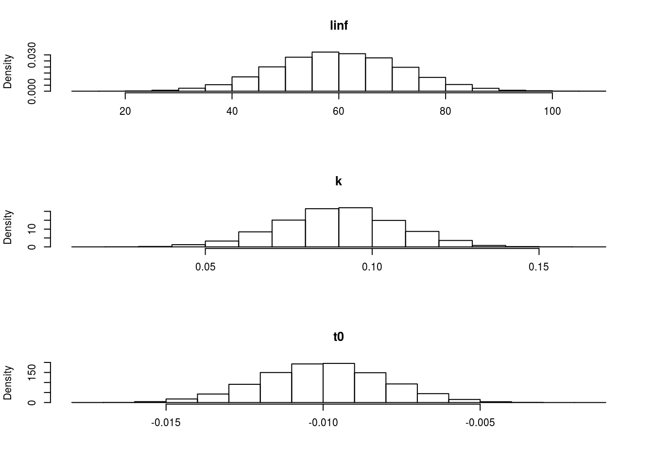
The marginal distributions of each of the parameters when using a multivariate normal distribution.
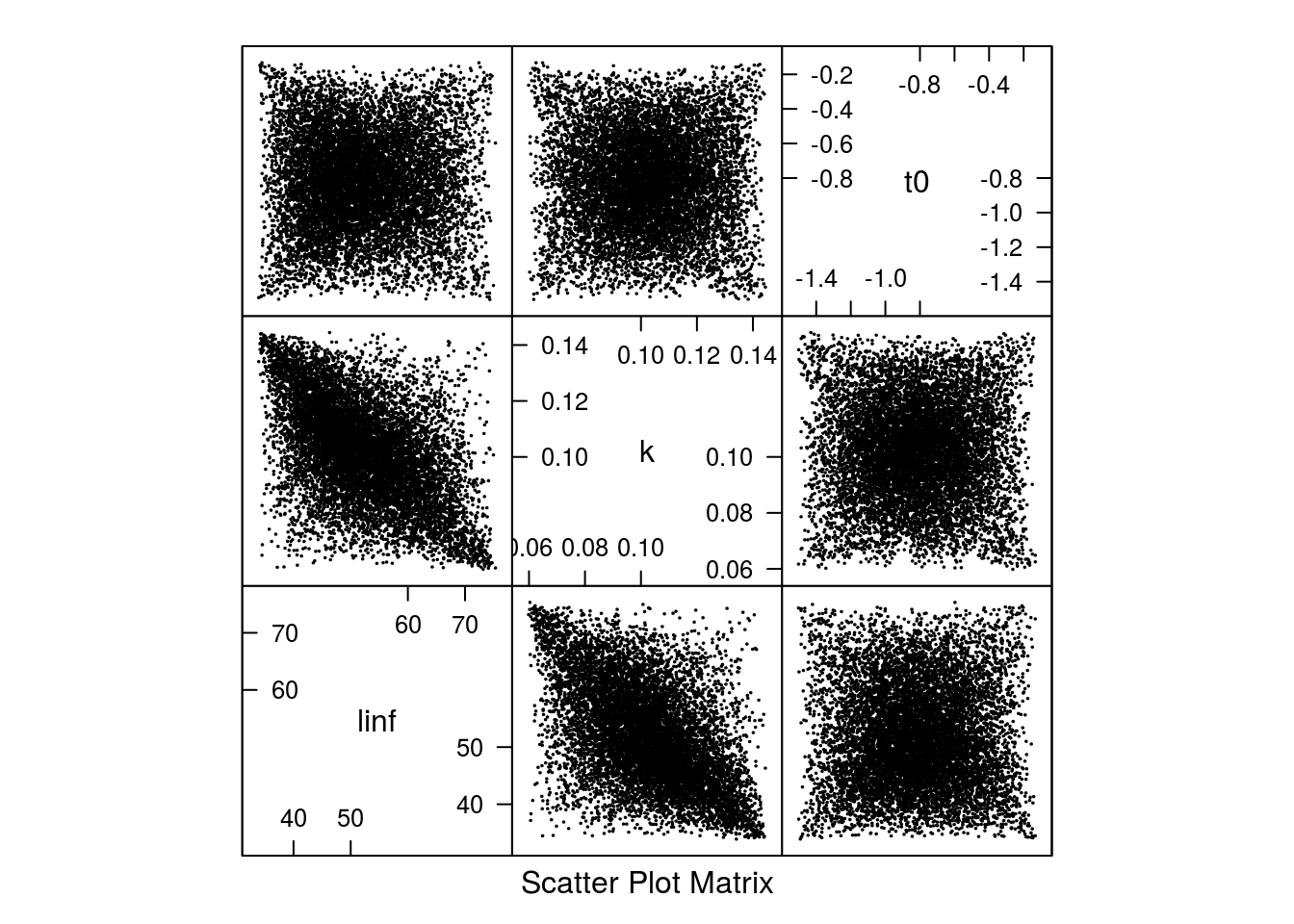
The shape of the correlation can be seen in Figure 2.
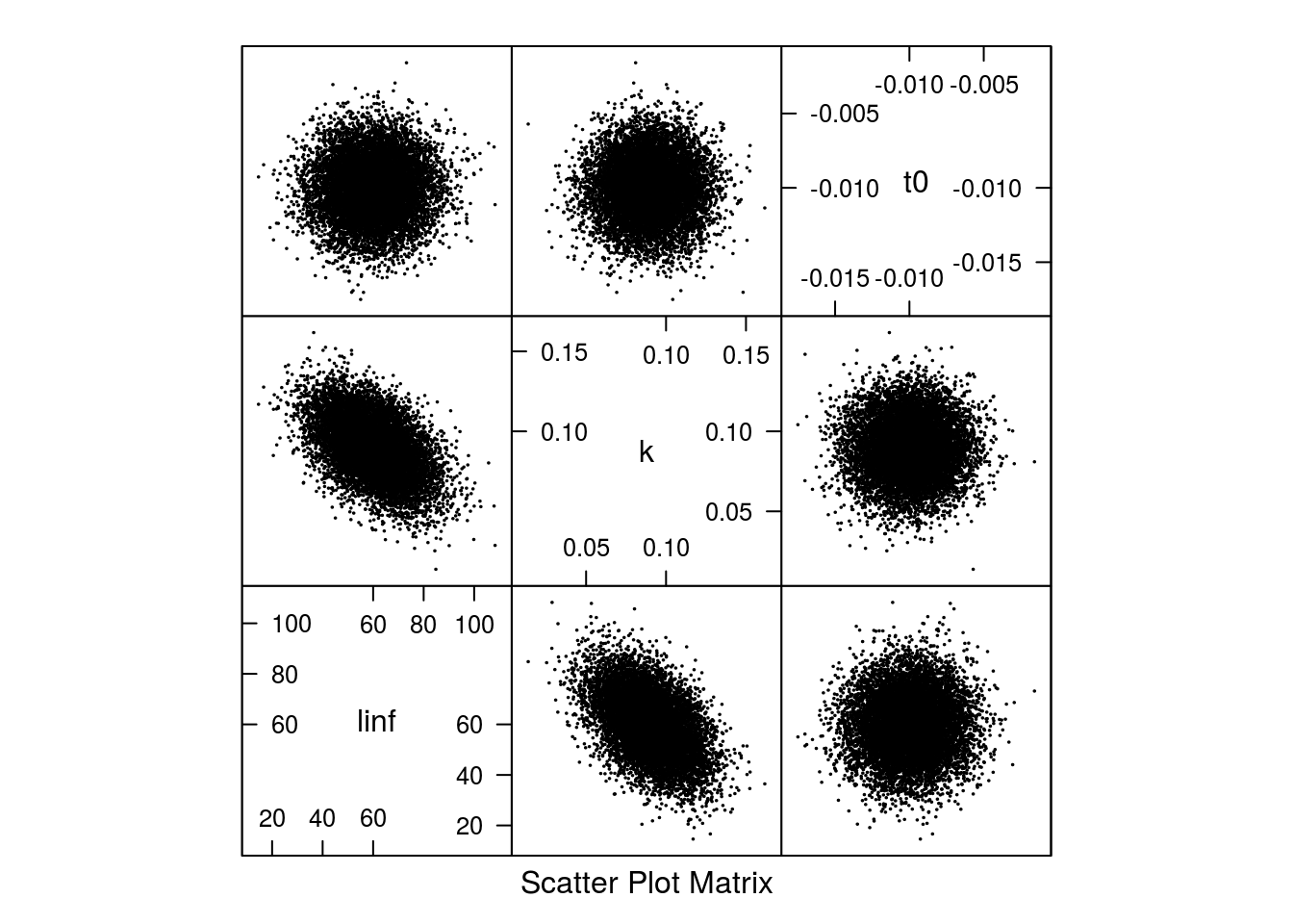
Scatter plot of the 10000 samples parameter from the multivariate normal distribution.
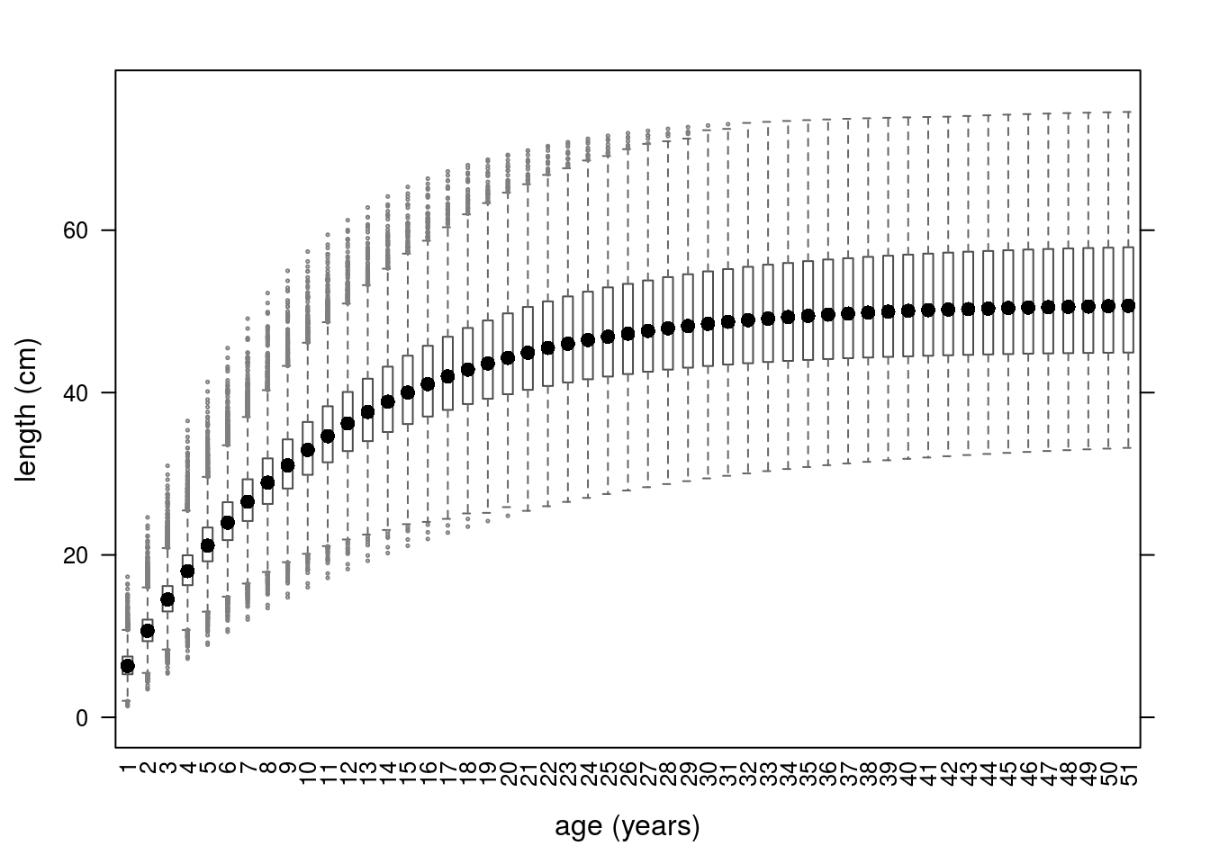
Growth curves for the 10000 iterations can be seen in Figure 3.
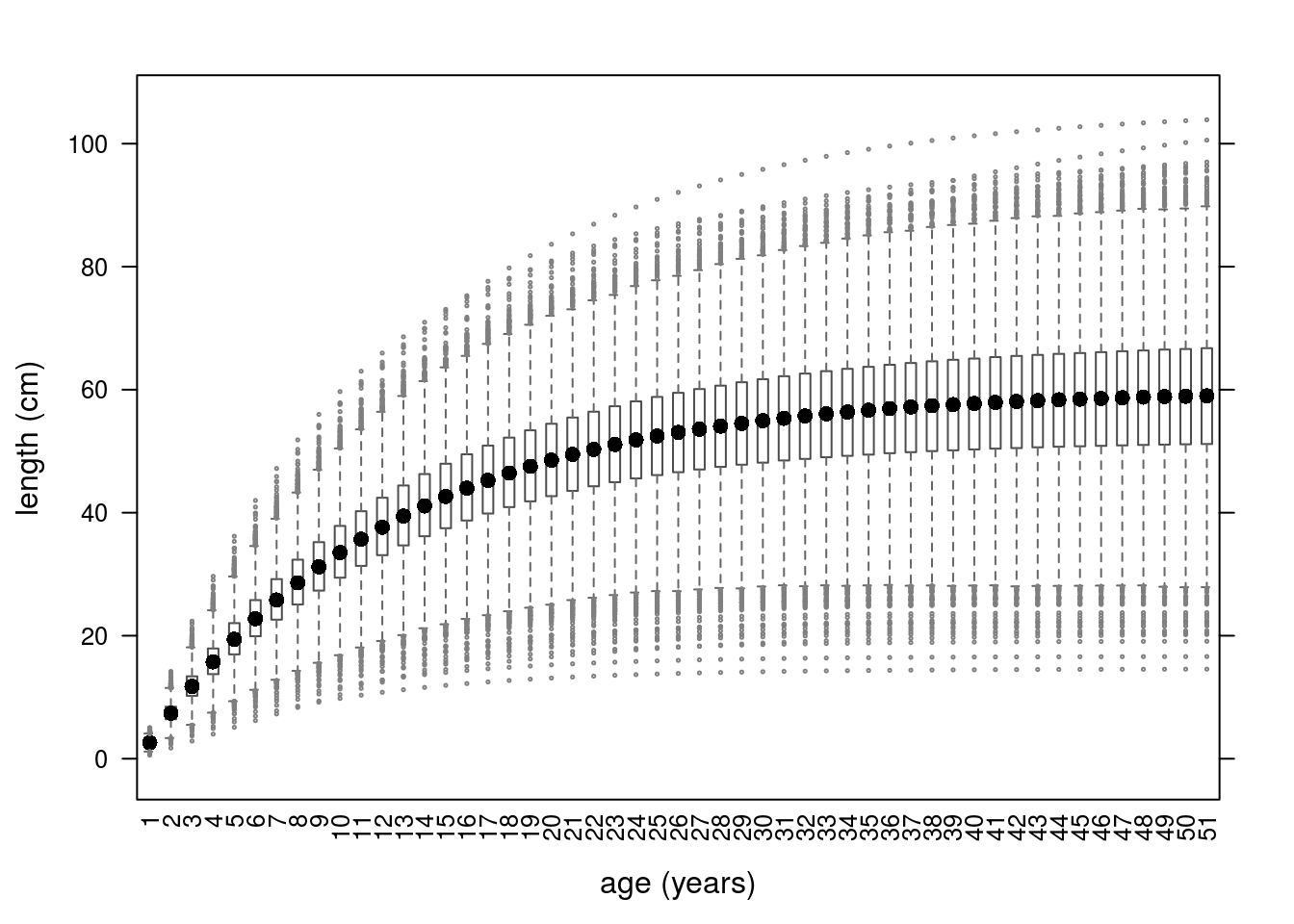
Growth curves using parameters simulated from a multivariate normal distribution.
Adding uncertainty to growth parameters with a multivariate triangle distribution
One alternative to using a normal distribution is to use a triangle distribution. We use the package triangle, where this distribution is parametrized using the minimum, maximum and median values. This can be very attractive if the analyst needs to, for example, obtain information from the web or literature and perform a meta-analysis.
Here we show an example of setting a triangle distribution with values taken from Fishbase. Note, this example needs an internet connection to access Fishbase.
# The web address for the growth parameters for redfish (Sebastes norvegicus)
addr <- 'http://www.fishbase.org/PopDyn/PopGrowthList.php?ID=501'
# Scrape the data
tab <- try(readHTMLTable(addr))
# Interrogate the data table and get vectors of the values
linf <- as.numeric(as.character(tab$dataTable[,2]))
k <- as.numeric(as.character(tab$dataTable[,4]))
t0 <- as.numeric(as.character(tab$dataTable[,5]))
# Set the min (a), max (b) and median (c) values for the parameter as a list of lists
# Note in this example that t0 has no 'c' (median) value which makes the distribution symmetrical
triPars <- list(list(a=min(linf), b=max(linf), c=median(linf)),
             list(a=min(k), b=max(k), c=median(k)),
             list(a=median(t0, na.rm=T)-IQR(t0, na.rm=T)/2, b=median(t0, na.rm=T)+
                    IQR(t0, na.rm=T)/2))
# Simulate 10000 times using mvrtriangle
vbTri <- mvrtriangle(10000, vbObj, paramMargins=triPars)
The marginals will reflect the uncertainty in the parameter values that were scraped from Fishbase but, because we don’t really believe the parameters are multivariate normal, here we adopted a distribution based on a t copula with triangle marginals.
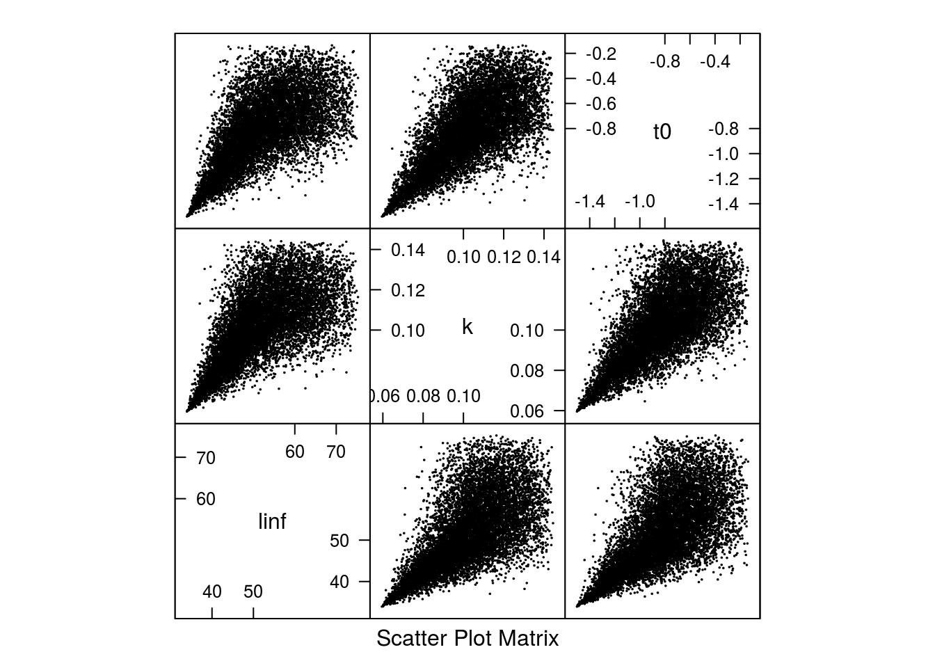
The marginal distributions can be seen in Figure 4 and the shape of the correlation can be seen in Figure 5.
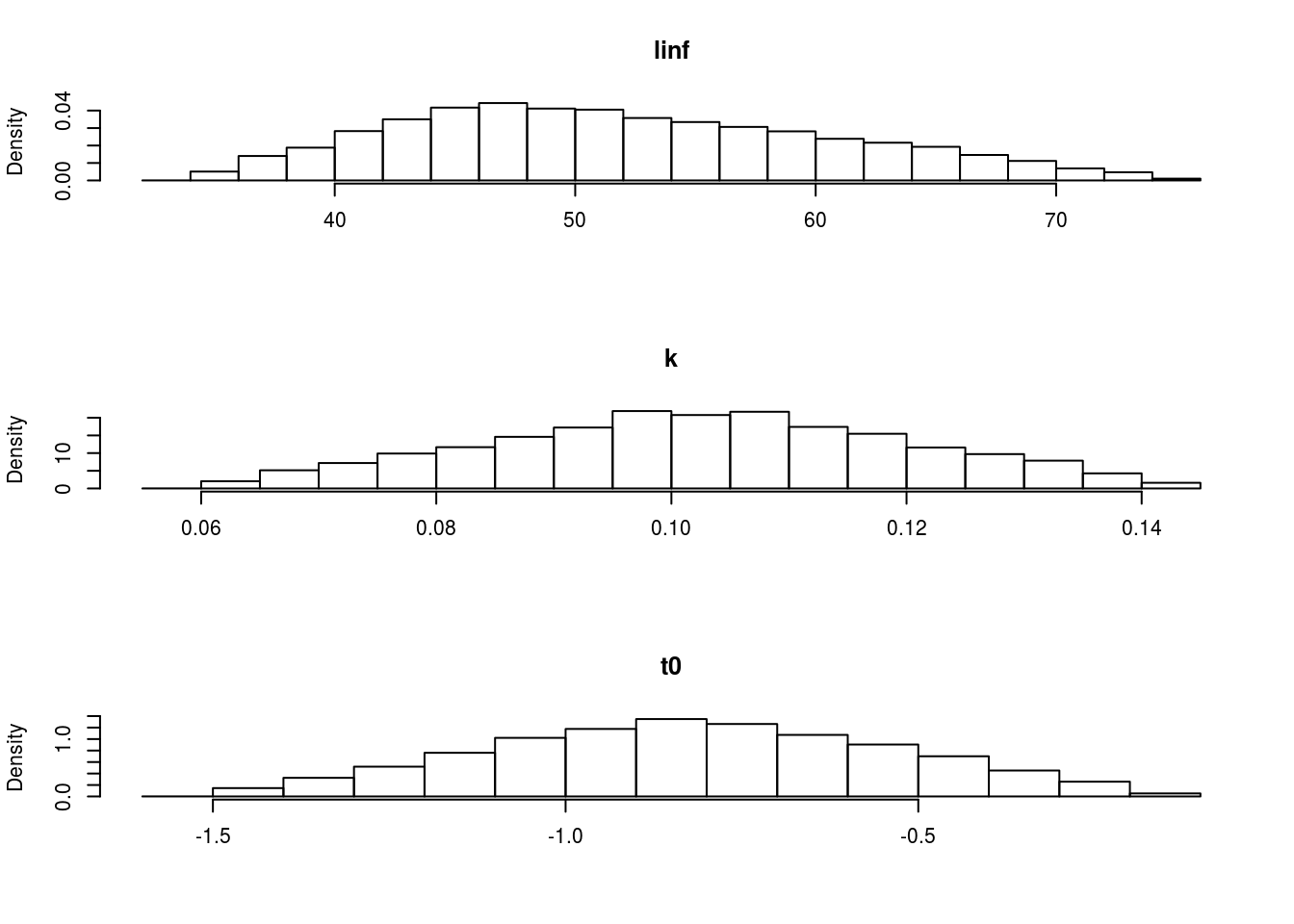
The marginal distributions of each of the parameters based on a multivariate triangle distribution.
Scatter plot of the 10000 parameter sets from the multivariate triangle distribution.
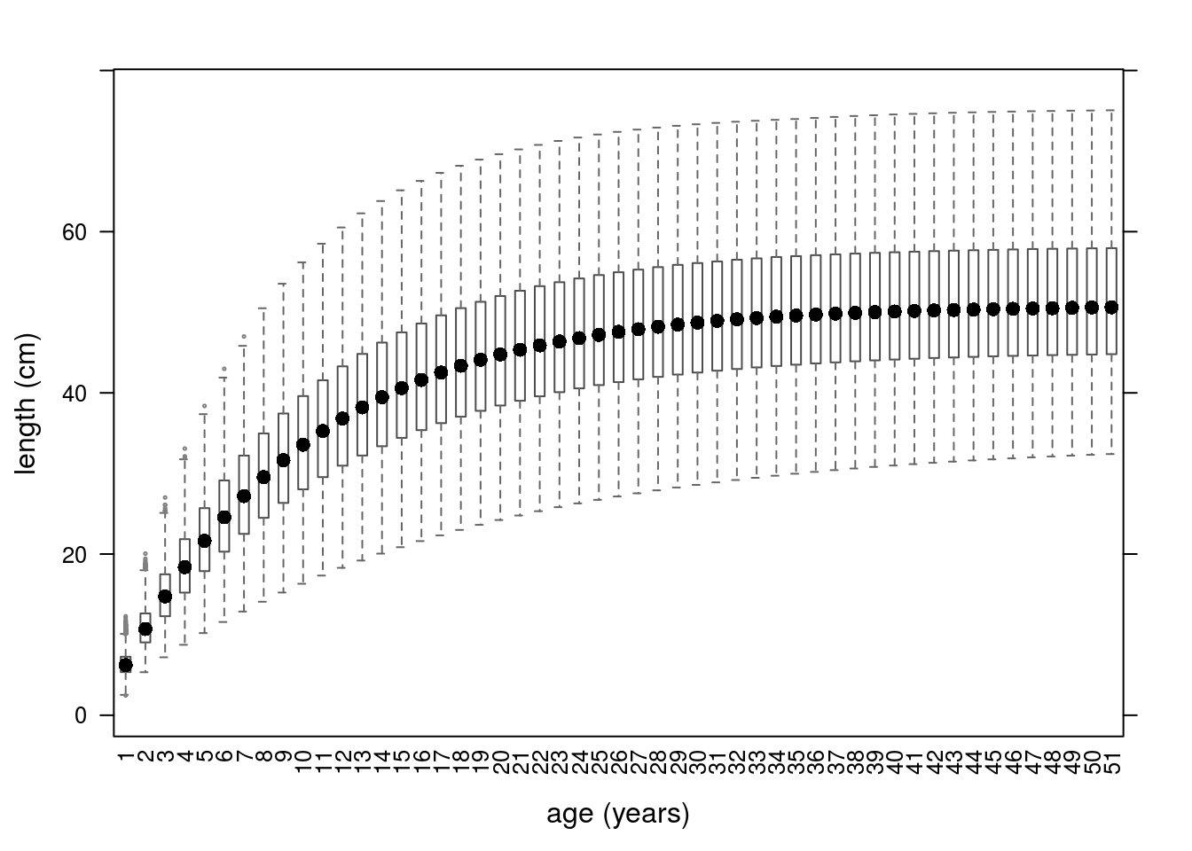
We can still use predict() to see the growth model uncertainty (Figure 6).
Growth curves using parameters simulated from a multivariate triangle distribution.
Note that the above examples use variance-covariance matrices that were made up. An alternative would be to scrape the entire growth parameters dataset from Fishbase and compute the shape of the variance-covariance matrix from this dataset.
Adding uncertainty to growth parameters with statistical copulas
A more general approach to adding parameter uncertainty is to make use of statistical copulas and marginal distributions of choice. This is possible with the mvrcop() function borrowed from the package copula. The example below keeps the same parameters and changes only the copula type and family, but a lot more can be done. Check the package copula for more information.
vbCop <- mvrcop(10000, vbObj, copula='archmCopula', family='clayton', param=2,
                margins='triangle', paramMargins=triPars)
The shape of the correlation changes is shown in (Figure 7) and the resulting growth curves in (Figure 8).
Scatter plot of the 10000 parameter sets based on the archmCopula copula with triangle margins.
Growth curves based on the archmCopula copula with triangle margins.
Converting from length to age based data - the l2a() method
After introducing uncertainty in the growth model through the parameters, we can transform the length-based dataset into an age-based one. The method that deals with this process is l2a(). The implementation of this method for the FLQuant class is the main workhorse. There are two other implementations, for the FLStock and FLIndex classes, which are mainly wrappers that call the FLQuant method several times.
When converting from length-based data to age-based data, we need to be aware of how the aggregation of length classes is performed. For example, individuals in length classes 1-2, 2-3, and 3-4 cm may all be considered age 1 fish (depending on the growth model). How should the values in those length classes be combined?
If the values are abundances, they should be summed. Summing other types of values, such as mean weight, does not make sense. Instead, these values are averaged over the length classes (possibly weighted by the abundance). This is controlled using the stat argument, which can either be mean or sum (the default). Fishing mortality is not computed to avoid making inappropriate assumptions about the meaning of F at length.
We demonstrate the method by converting a catch-at-length FLQuant to a catch-at-age FLQuant. First we make an a4aGr object with a multivariate triangle distribution (using the parameters we derive above). We use 10 iterations as an example, and call l2a() by passing it the length-based FLQuant and the a4aGr object.
vbTriSmall <- mvrtriangle(10, vbObj, paramMargins=triPars)
cth.n <- l2a(catch.n(rfLen.stk), vbTriSmall)dim(cth.n)[1] 78 26 1 4 1 10In the previous example, the FLQuant object that was sliced (catch.n(rfLen.stk)) had only one iteration. This iteration was sliced by each of the iterations in the growth model. It is possible for the FLQuant object to have the same number of iterations as the growth model, in which case each iteration of the FLQuant and the growth model are used together. It is also possible for the growth model to have only one iteration while the FLQuant object has many iterations. The same growth model is then used for each of the FLQuant iterations. As with all FLR objects, the general rule is one or n iterations.
As well as converting one FLQuant at a time, we can convert entire FLStock and FLIndex objects. In these cases, the individual FLQuant slots of those classes are converted from length to age. As mentioned above, the aggregation method depends on the types of value the slots contain. The abundance slots (.n, such as stock.n) are summed. The wt, m, mat, harvest.spwn and m.spwn slots of an FLStock object are averaged. The catch.wt and sel.pattern slots of an FLIndex object are averaged, while the index, index.var and catch.n slots are summed.
The method for FLStock classes takes an additional argument for the plusgroup.
aStk <- l2a(rfLen.stk, vbTriSmall, plusgroup=14)Warning in .local(object, model, ...): Individual weights, M and maturity will be (weighted) averaged accross lengths,
harvest is not computed and everything else will be summed.
If this is not what you want, you'll have to deal with these slots by hand.Warning in .local(object, model, ...): Some ages are less than 0, indicating a mismatch between input data lengths
and growth parameters (possibly t0)Warning in .local(object, model, ...): Trimming age range to a minimum of 0[1] "maxfbar has been changed to accomodate new plusgroup"aIdx <- l2a(rfTrawl.idx, vbTriSmall)Warning in l2a(rfTrawl.idx, vbTriSmall): Some ages are less than 0, indicating a mismatch between input data lengths
and growth parameters (possibly t0)Warning in l2a(rfTrawl.idx, vbTriSmall): Trimming age range to a minimum of
0When converting with l2a() all lengths above Linf are converted to the maximum age, because there is no information in the growth model about how to deal with individuals larger than Linf.
References
Ernesto Jardim, Colin P. Millar, Iago Mosqueira, Finlay Scott, Giacomo Chato Osio, Marco Ferretti, Nekane Alzorriz, Alessandro Orio; What if stock assessment is as simple as a linear model? The a4a initiative. ICES J Mar Sci 2015; 72 (1): 232-236. DOI: https://doi.org/10.1093/icesjms/fsu050
Colin P. Millar, Ernesto Jardim, Finlay Scott, Giacomo Chato Osio, Iago Mosqueira, Nekane Alzorriz; Model averaging to streamline the stock assessment process. ICES J Mar Sci 2015; 72 (1): 93-98. DOI: https://doi.org/10.1093/icesjms/fsu043
Scott F, Jardim E, Millar CP, Cervino S (2016) An Applied Framework for Incorporating Multiple Sources of Uncertainty in Fisheries Stock Assessments. PLoS ONE 11(5): e0154922. DOI: https://doi.org/10.1371/journal.pone.0154922
More information
Documentation can be found at (http://flr-project.org/FLa4a). You are welcome to:
- Submit suggestions and bug-reports at: (https://github.com/flr/FLa4a/issues)
- Send a pull request on: (https://github.com/flr/FLa4a/)
- Compose a friendly e-mail to the maintainer, see
packageDescription('FLa4a')
Software Versions
- R version 3.4.1 (2017-06-30)
- FLCore: 2.6.5
- FLa4a: 1.1.3
- Compiled: Fri Sep 15 15:46:57 2017
License
This document is licensed under the Creative Commons Attribution-ShareAlike 4.0 International license.