Natural Mortality Modelling
Assessment for All initiative (a4a)
18 September, 2017
The document explains the approach being developed by a4a to integrate uncertainty in natural mortality into stock assessment and advice. It presents a mixture of text and code, where the former explains the concepts behind the methods, while the latter shows how these can be run with the software provided.
Required packages
To follow this tutorial you should have installed the following packages:
You can do so as follows,
install.packages(c("copula","triangle", "coda", "XML", "reshape2", "latticeExtra"))
# from FLR
install.packages(c("FLCore", "FLa4a"), repos="http://flr-project.org/R")
# Load all necessary packages and datasets, trim pkg messages
library(FLa4a)
library(XML)
library(reshape2)
library(latticeExtra)
data(ple4)
data(ple4.indices)
data(ple4.index)
data(rfLen)Background
In a4a, natural mortality is dealt with as an external parameter to the stock assessment model. The rationale for modelling natural mortality is similar to that for growth: one should be able to obtain information from a range of sources and feed it into the assessment.
The mechanism used by a4a is to build an interface that is transparent and flexible, and makes it easy to explore different options. In relation to natural mortality, it means that the analyst should be able to use distinct models like Gislasson’s, Charnov’s, Pauly’s, etc., in a coherent framework, making it possible to compare the outcomes of the assessment.
Within the a4a framework, the general method for inserting natural mortality in the stock assessment is to:
- Create an object of class
a4aMwhich holds the natural mortality model and parameters. - Add uncertainty to the parameters in the
a4aMobject. - Apply the
m()method to thea4aMobject to create an age or length basedFLQuantobject of the required dimensions.
The resulting FLQuant object can then be directly inserted into an FLStock object to be used for the assessment.
In this section we go through each of the steps in detail using a variety of different models.
For more information on the a4a methodologies refer to Jardim, et.al, 2014, Millar, et.al, 2014 and Scott, et.al, 2016.
a4aM - The M class
Natural mortality is implemented in a class named a4aM. This class is made up of three objects of the class FLModelSim. Each object is a model that represents one effect: an age or length effect, a scaling (level) effect and a time trend, named shape, level and trend, respectively. The impact of the models is multiplicative, i.e. the overal natural mortality is given by shape x level x trend. Check the help files for more information.
showClass("a4aM")Class "a4aM" [package "FLa4a"]
Slots:
Name: shape level trend name desc range
Class: FLModelSim FLModelSim FLModelSim character character numeric
Extends: "FLComp"The a4aM constructor requires that the models and parameters are provided. The default method will build each of these models as a constant value of 1.
As a simple example, the usual “0.2” guesstimate could be set up by setting the level model to have a single parameter with a fixed value, while the other two models, shape and trend, have a default value of 1 (meaning that they have no effect).
mod02 <- FLModelSim(model=~a, params=FLPar(a=0.2))
m1 <- a4aM(level=mod02)
m1
a4aM object:
shape: ~1
level: ~a
trend: ~1More interesting natural mortality shapes can be set up using biological knowledge. The following example uses an exponential decay over ages (implying that the resulting FLQuant generated by the m() method will be age based). We also use Jensen’s second estimator Kenchington, 2013 as a scaling level model, which is based on the von Bertalanffy \(k\) parameter, \(M=1.5k\).
shape2 <- FLModelSim(model=~exp(-age-0.5))
level2 <- FLModelSim(model=~1.5*k, params=FLPar(k=0.4))
m2 <- a4aM(shape=shape2, level=level2)
m2
a4aM object:
shape: ~exp(-age - 0.5)
level: ~1.5 * k
trend: ~1Note that the shape model has age as a parameter, but is not set using the params argument.
The shape model does not have to be age-based. For example, here we set up a shape model using Gislason’s second estimator Kenchington, 2013: \(M_l=K(\frac{L_{\inf}}{l})^{1.5}\). We use the default level and trend models. The current m() method is not ideal for length-based methods because you cannot specify length ranges and half-widths to make compatible with FLStockLen
shape_len <- FLModelSim(model=~k*(linf/len)^1.5, params=FLPar(linf=60, k=0.4))
m_len <- a4aM(shape=shape_len)
Another option is to model how an external factor may impact the natural mortality. This can be added through the trend model. Suppose natural mortality can be modelled with a dependency on the NAO index, due to some mechanism that results in having lower mortality when NAO is negative and higher when it’s positive. In this example, the impact is represented by the NAO value in the quarter before spawning, which occurs in the second quarter.
We use this to make a complicated natural mortality model with an age based shape model, a level model based on \(k\) and a trend model driven by NAO, where mortality increases by 50% if NAO is positive in the first quarter. Note, this example needs an internet connection to access the NAO data.
# Get NAO
nao.orig <- read.table("https://www.esrl.noaa.gov/psd/data/correlation/nao.data", skip=1, nrow=62, na.strings="-99.90")
dnms <- list(quant="nao", year=1948:2009, unit="unique", season=1:12, area="unique")
# Build an FLQuant from the NAO data, with the season slot representing months
nao.flq <- FLQuant(unlist(nao.orig[,-1]), dimnames=dnms, units="nao")
# Build covar by calculating the mean over the first 3 months
nao <- seasonMeans(nao.flq[,,,1:3])
# Turn into Boolean
nao <- (nao>0)
# Constructor
trend3 <- FLModelSim(model=~1+b*nao, params=FLPar(b=0.5))
shape3 <- FLModelSim(model=~exp(-age-0.5))
level3 <- FLModelSim(model=~1.5*k, params=FLPar(k=0.4))
m3 <- a4aM(shape=shape3, level=level3, trend=trend3)
m3
a4aM object:
shape: ~exp(-age - 0.5)
level: ~1.5 * k
trend: ~1 + b * naoAdding uncertainty to natural mortality parameters with a multivariate normal distribution
Uncertainty in natural mortality is added through uncertainty in the parameters.
In this section we’ll show how to add multivariate normal uncertainty. We make use of method mvrnorm() from class FLModelSim, which is a wrapper for the method mvrnorm() distributed by the package MASS.
We’ll create an a4aM object with an exponential shape, a level model based on \(k\) and temperature (Jensen’s third estimator), and a trend model driven by the NAO (as above). Afterwards, a variance-covariance matrix for the level and trend models will be included. Finally, we create an object with 100 iterations using the mvrnorm() method.
# Create the object using shape, level and trend models
shape4 <- FLModelSim(model=~exp(-age-0.5))
level4 <- FLModelSim(model=~k^0.66*t^0.57, params=FLPar(k=0.4, t=10), vcov=array(c(0.002, 0.01, 0.01, 1), dim=c(2,2)))
trend4 <- FLModelSim(model=~1+b*nao, params=FLPar(b=0.5), vcov=matrix(0.02))
m4 <- a4aM(shape=shape4, level=level4, trend=trend4)
# Call mvrnorm()
m4 <- mvrnorm(100, m4)
m4
a4aM object:
shape: ~exp(-age - 0.5)
level: ~k^0.66 * t^0.57
trend: ~1 + b * nao# Inspect the models (e.g. level)
level(m4) #can also be done with m4@levelAn object of class "FLModelSim"
Slot "model":
~k^0.66 * t^0.57
<environment: 0x2d97d18>
Slot "params":
An object of class "FLPar"
iters: 100
params
k t
0.39811(0.0457) 9.87074(0.8623)
units: NA
Slot "vcov":
[,1] [,2]
[1,] 0.002 0.01
[2,] 0.010 1.00
Slot "distr":
[1] "norm"# Note the variance in the parameters (e.g. trend)
params(trend(m4))An object of class "FLPar"
iters: 100
params
b
0.50488(0.136)
units: NA # Note the shape model has no parameters and no uncertainty
params(shape(m4))An object of class "FLPar"
[1] NA
units: NA In this particular case, the shape model will not be randomized because it doesn’t have a variance-covariance matrix. Also note that because there is only one parameter in the trend model, the randomisation will use a univariate normal distribution.
The same model could be achieved by using mvrnorm() on each model component:
m4 <- a4aM(shape=shape4, level=mvrnorm(100, level4), trend=mvrnorm(100, trend4))%Note: How to include ageing error ???
Adding uncertainty to natural mortality parameters with statistical copulas
We can also use copulas to add parameter uncertainty to the natural mortality model, similar to the way we use them for the growth model. Using a triangle distribution. We use the package triangle, where this distribution is parametrized using the minimum, maximum and median values. This can be very attractive if the analyst needs to, for example, obtain information from the web or literature and perform a meta-analysis. As stated above, these processes make use of the methods implemented for the FLModelSim class.
In the following example, we’ll use Gislason’s second estimator, \(M_l=K(\frac{L_{\inf}}{l})^{1.5}\), and a triangle copula to model parameter uncertainty. The method mvrtriangle() is used to create 1000 iterations.
linf <- 60
k <- 0.4
# vcov matrix (make up some values)
mm <- matrix(NA, ncol=2, nrow=2)
# calculate variances assuming a 10% cv
diag(mm) <- c((linf*0.1)^2, (k*0.1)^2)
# calculate covariances assuming a correlation of 0.2
mm[upper.tri(mm)] <- mm[lower.tri(mm)] <- sqrt(prod(diag(mm)))*0.2
# a good way to check is using cov2cor
cov2cor(mm)| 1.0 | 0.2 |
| 0.2 | 1.0 |
# create the FLModelSim object
mgis2 <- FLModelSim(model=~k*(linf/len)^1.5, params=FLPar(linf=linf, k=k), vcov=mm)
# set the lower (a), upper (b) and (optionally) centre (c) of the parameters linf and k (note, without the centre, the triangle is symmetrical)
pars <- list(list(a=55,b=65), list(a=0.3, b=0.6, c=0.35))
# generate 1000 sample sets using mvrtriangle
mgis2 <- mvrtriangle(1000, mgis2, paramMargins=pars)
mgis2
An object of class "FLModelSim"
Slot "model":
~k * (linf/len)^1.5
<environment: 0x2d97d18>
Slot "params":
An object of class "FLPar"
iters: 1000
params
linf k
59.94387(2.1843) 0.41208(0.0749)
units: NA
Slot "vcov":
[,1] [,2]
[1,] 36.000 0.0480
[2,] 0.048 0.0016
Slot "distr":
[1] "un <deprecated slot> triangle"The resulting parameter estimates and marginal distributions can be seen in Figure 1 and Figure 2.
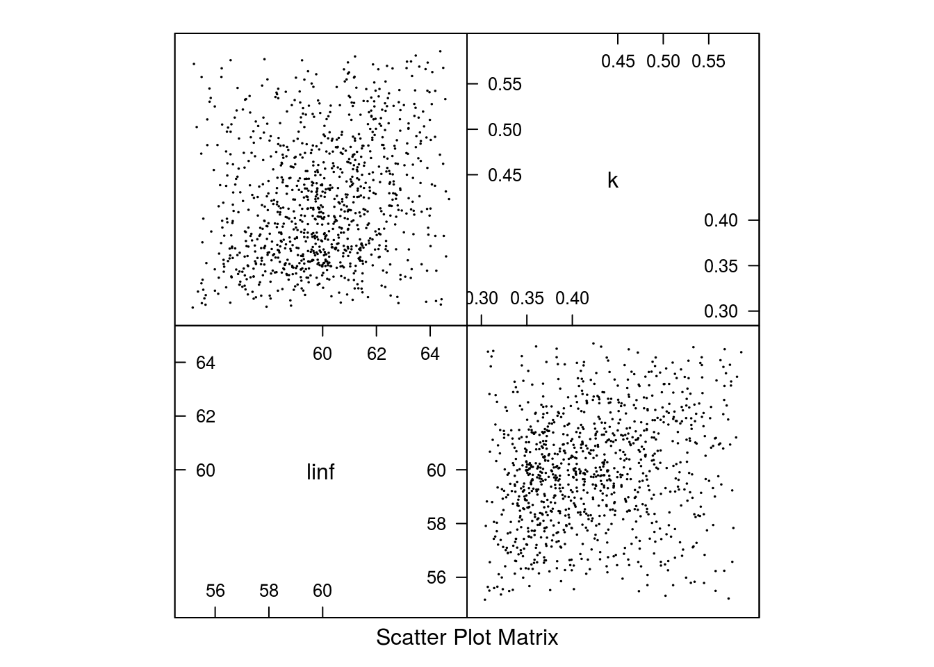
Parameter estimates for Gislason’s second natural mortality model based on a triangle distribution.
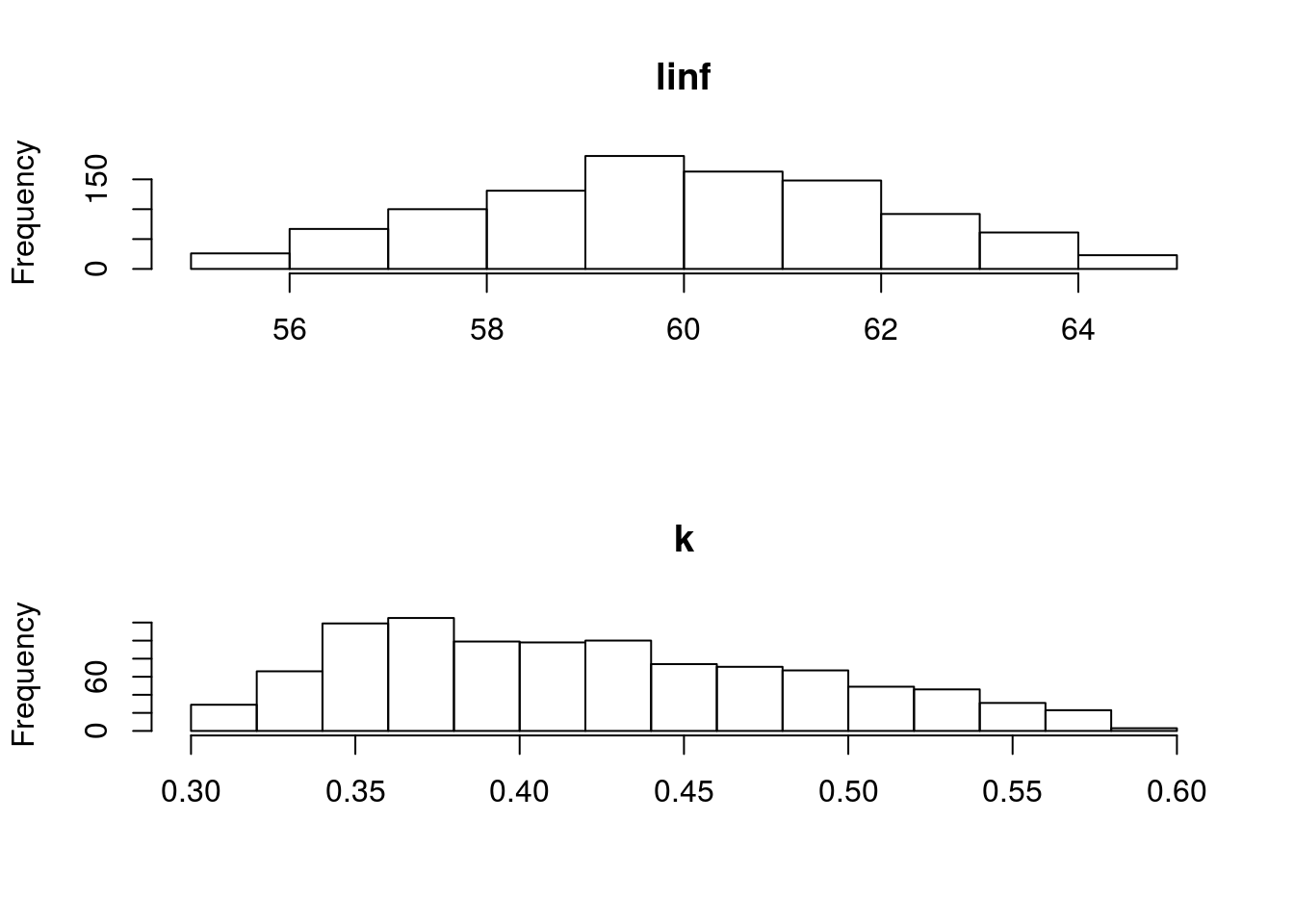
Marginal distributions of the parameters for Gislason’s second natural mortality model using a triangle distribution.
We now have a new model that can be used for the shape model. You can use the constructor or the set method to add the new model. Note that we have quite a complex method now for M. A length based shape model from Gislason’s work, Jensen’s third model based on temperature level and a time trend depending on an environmental index, NAO. All of the component models have uncertainty in their parameters.
#Using the constructor
m5 <- a4aM(shape=mgis2, level=level4, trend=trend4)
# or the set method for shape to change m4 previously created
m5 <- m4
shape(m5) <- mgis2
Computing natural mortality time series - the m() method
Now that we have set up the natural mortality a4aM model and added parameter uncertainty to each component, we are ready to generate the FLQuant for natural mortality. For that we need the m() method.
The m() method is the workhorse method for computing natural mortality. The method returns an FLQuant that can be inserted in an FLStock for usage by the assessment method.
The method uses the range slot to work out the dimensions of the FLQuant object. % Future developments will also allow for easy insertion into FLStockLen objects.
The size of the FLQuant object is determined by the min, max, minyear and maxyear elements of the range slot of the a4aM object. By default the values of these elements are set to 0, giving an FLQuant with length 1 in the quant and year dimension. The range slot can be set by hand, or by using the rngquant() and rngyear() methods.
The name of the first dimension of the output FLQuant (e.g. ‘age’ or ‘len’) is determined by the parameters of the shape model. If it is not clear what the name should be then the name is set to ‘quant’.
Here we demonstrate m() using the simple a4aM object we created above that has constant natural mortality.
# Start with the simplest model
m1
a4aM object:
shape: ~1
level: ~a
trend: ~1# Check the range
range(m1) # no ages or years... min max plusgroup minyear maxyear minmbar maxmbar
0 0 0 0 0 0 0 m(m1) # confirms no ages or yearsAn object of class "FLQuant"
An object of class "FLQuant"
, , unit = unique, season = all, area = unique
year
quant 0
0 0.2
units: NA # Set the quant and year ranges
range(m1, c('min', 'max')) <- c(0,7) # set the quant range
range(m1, c('minyear', 'maxyear')) <- c(2000, 2010) # set the year range
range(m1) min max plusgroup minyear maxyear minmbar maxmbar
0 7 0 2000 2010 0 0 # Show the object with the M estimates by age and year
# (note the name of the first dimension is 'quant')
m(m1)An object of class "FLQuant"
, , unit = unique, season = all, area = unique
year
quant 2000 2001 2002 2003 2004
0 0.2 0.2 0.2 0.2 0.2
1 0.2 0.2 0.2 0.2 0.2
2 0.2 0.2 0.2 0.2 0.2
3 0.2 0.2 0.2 0.2 0.2
4 0.2 0.2 0.2 0.2 0.2
5 0.2 0.2 0.2 0.2 0.2
6 0.2 0.2 0.2 0.2 0.2
7 0.2 0.2 0.2 0.2 0.2
[ ... 1 years]
year
quant 2006 2007 2008 2009 2010
0 0.2 0.2 0.2 0.2 0.2
1 0.2 0.2 0.2 0.2 0.2
2 0.2 0.2 0.2 0.2 0.2
3 0.2 0.2 0.2 0.2 0.2
4 0.2 0.2 0.2 0.2 0.2
5 0.2 0.2 0.2 0.2 0.2
6 0.2 0.2 0.2 0.2 0.2
7 0.2 0.2 0.2 0.2 0.2 The next example has an age-based shape. As the shape model has ‘age’ as a variable which is not included in the FLPar slot, it is used as the name of the first dimension of the resulting FLQuant. Note that in this case, the mbar values in the range become relevant, once that mbar is used to compute the mean level. This mean level will match the value given by the level model. The mbar range can be changed with the rngmbar() method. We illustrate this by making an FLQuant with age-varying natural mortality.
# Check the model and set the ranges
m2
a4aM object:
shape: ~exp(-age - 0.5)
level: ~1.5 * k
trend: ~1range(m2, c('min', 'max')) <- c(0,7) # set the quant range
range(m2, c('minyear', 'maxyear')) <- c(2000, 2010) # set the year range
range(m2) min max plusgroup minyear maxyear minmbar maxmbar
0 7 0 2000 2010 0 0 m(m2)An object of class "FLQuant"
, , unit = unique, season = all, area = unique
year
age 2000 2001 2002 2003 2004
0 0.60000000 0.60000000 0.60000000 0.60000000 0.60000000
1 0.22072766 0.22072766 0.22072766 0.22072766 0.22072766
2 0.08120117 0.08120117 0.08120117 0.08120117 0.08120117
3 0.02987224 0.02987224 0.02987224 0.02987224 0.02987224
4 0.01098938 0.01098938 0.01098938 0.01098938 0.01098938
5 0.00404277 0.00404277 0.00404277 0.00404277 0.00404277
6 0.00148725 0.00148725 0.00148725 0.00148725 0.00148725
7 0.00054713 0.00054713 0.00054713 0.00054713 0.00054713
[ ... 1 years]
year
age 2006 2007 2008 2009 2010
0 0.60000000 0.60000000 0.60000000 0.60000000 0.60000000
1 0.22072766 0.22072766 0.22072766 0.22072766 0.22072766
2 0.08120117 0.08120117 0.08120117 0.08120117 0.08120117
3 0.02987224 0.02987224 0.02987224 0.02987224 0.02987224
4 0.01098938 0.01098938 0.01098938 0.01098938 0.01098938
5 0.00404277 0.00404277 0.00404277 0.00404277 0.00404277
6 0.00148725 0.00148725 0.00148725 0.00148725 0.00148725
7 0.00054713 0.00054713 0.00054713 0.00054713 0.00054713# Note that the level value is
c(predict(level(m2)))[1] 0.6# which is the same as
m(m2)["0"]An object of class "FLQuant"
, , unit = unique, season = all, area = unique
year
age 2000 2001 2002 2003 2004
0 0.6 0.6 0.6 0.6 0.6
[ ... 1 years]
year
age 2006 2007 2008 2009 2010
0 0.6 0.6 0.6 0.6 0.6 # This is because the mbar range is currently set to "0" and "0" (see above)
# and the mean natural mortality value over this range is given by the level model.
# We can change the mbar range
range(m2, c('minmbar', 'maxmbar')) <- c(0,7) # set the quant range
range(m2) min max plusgroup minyear maxyear minmbar maxmbar
0 7 0 2000 2010 0 7 # which rescales the the natural mortality at age
m(m2)An object of class "FLQuant"
, , unit = unique, season = all, area = unique
year
age 2000 2001 2002 2003 2004
0 3.0351969 3.0351969 3.0351969 3.0351969 3.0351969
1 1.1165865 1.1165865 1.1165865 1.1165865 1.1165865
2 0.4107692 0.4107692 0.4107692 0.4107692 0.4107692
3 0.1511136 0.1511136 0.1511136 0.1511136 0.1511136
4 0.0555916 0.0555916 0.0555916 0.0555916 0.0555916
5 0.0204510 0.0204510 0.0204510 0.0204510 0.0204510
6 0.0075235 0.0075235 0.0075235 0.0075235 0.0075235
7 0.0027677 0.0027677 0.0027677 0.0027677 0.0027677
[ ... 1 years]
year
age 2006 2007 2008 2009 2010
0 3.0351969 3.0351969 3.0351969 3.0351969 3.0351969
1 1.1165865 1.1165865 1.1165865 1.1165865 1.1165865
2 0.4107692 0.4107692 0.4107692 0.4107692 0.4107692
3 0.1511136 0.1511136 0.1511136 0.1511136 0.1511136
4 0.0555916 0.0555916 0.0555916 0.0555916 0.0555916
5 0.0204510 0.0204510 0.0204510 0.0204510 0.0204510
6 0.0075235 0.0075235 0.0075235 0.0075235 0.0075235
7 0.0027677 0.0027677 0.0027677 0.0027677 0.0027677# Check that the mortality over the mean range is the same as the level model
quantMeans(m(m2)[as.character(0:5)])An object of class "FLQuant"
, , unit = unique, season = all, area = unique
year
age 2000 2001 2002 2003 2004
all 0.79828 0.79828 0.79828 0.79828 0.79828
[ ... 1 years]
year
age 2006 2007 2008 2009 2010
all 0.79828 0.79828 0.79828 0.79828 0.79828The next example uses a time trend for the trend model. We use the m3 model we derived earlier. The trend model for this model has a covariate, ‘nao’. This needs to be passed to the m() method. The year range of the ‘nao’ covariate should match that of the range slot.
# Pass in a single nao value (only one year, because the trend model needs
# at least one value)
m(m3, nao=1)
An object of class "FLQuant"
An object of class "FLQuant"
, , unit = unique, season = all, area = unique
year
age 0
0 0.9
units: NA # Set ages
range(m3, c('min', 'max')) <- c(0,7) # set the quant range
m(m3, nao=0)An object of class "FLQuant"
An object of class "FLQuant"
, , unit = unique, season = all, area = unique
year
age 0
0 0.60000000
1 0.22072766
2 0.08120117
3 0.02987224
4 0.01098938
5 0.00404277
6 0.00148725
7 0.00054713
units: NA # With ages and years - passing in the NAO data as numeric (1,0,1,0)
range(m3, c('minyear', 'maxyear')) <- c(2000, 2003) # set the year range
m(m3, nao=as.numeric(nao[,as.character(2000:2003)]))An object of class "FLQuant"
An object of class "FLQuant"
, , unit = unique, season = all, area = unique
year
age 2000 2001 2002 2003
0 0.90000000 0.60000000 0.90000000 0.60000000
1 0.33109150 0.22072766 0.33109150 0.22072766
2 0.12180175 0.08120117 0.12180175 0.08120117
3 0.04480836 0.02987224 0.04480836 0.02987224
4 0.01648407 0.01098938 0.01648407 0.01098938
5 0.00606415 0.00404277 0.00606415 0.00404277
6 0.00223088 0.00148725 0.00223088 0.00148725
7 0.00082069 0.00054713 0.00082069 0.00054713
units: NA The final example show how m() can be used to make an FLQuant with uncertainty (see Figure 3). We use the m4 object from earlier with uncertainty on the level and trend parameters.
range(m4, c('min', 'max')) <- c(0,7)             # set the quant range
range(m4, c('minyear', 'maxyear')) <- c(2000, 2003)
flq <- m(m4, nao=as.numeric(nao[,as.character(2000:2003)]))
flq
An object of class "FLQuant"
An object of class "FLQuant"
iters: 100
, , unit = unique, season = all, area = unique
year
age 2000 2001 2002
0 3.0079919(0.359714) 2.0389830(0.229792) 3.0079919(0.359714)
1 1.1065784(0.132331) 0.7500999(0.084536) 1.1065784(0.132331)
2 0.4070874(0.048682) 0.2759463(0.031099) 0.4070874(0.048682)
3 0.1497591(0.017909) 0.1015150(0.011441) 0.1497591(0.017909)
4 0.0550933(0.006588) 0.0373453(0.004209) 0.0550933(0.006588)
5 0.0202677(0.002424) 0.0137386(0.001548) 0.0202677(0.002424)
6 0.0074561(0.000892) 0.0050541(0.000570) 0.0074561(0.000892)
7 0.0027429(0.000328) 0.0018593(0.000210) 0.0027429(0.000328)
year
age 2003
0 2.0389830(0.229792)
1 0.7500999(0.084536)
2 0.2759463(0.031099)
3 0.1015150(0.011441)
4 0.0373453(0.004209)
5 0.0137386(0.001548)
6 0.0050541(0.000570)
7 0.0018593(0.000210)
units: NA dim(flq)[1] 8 4 1 1 1 100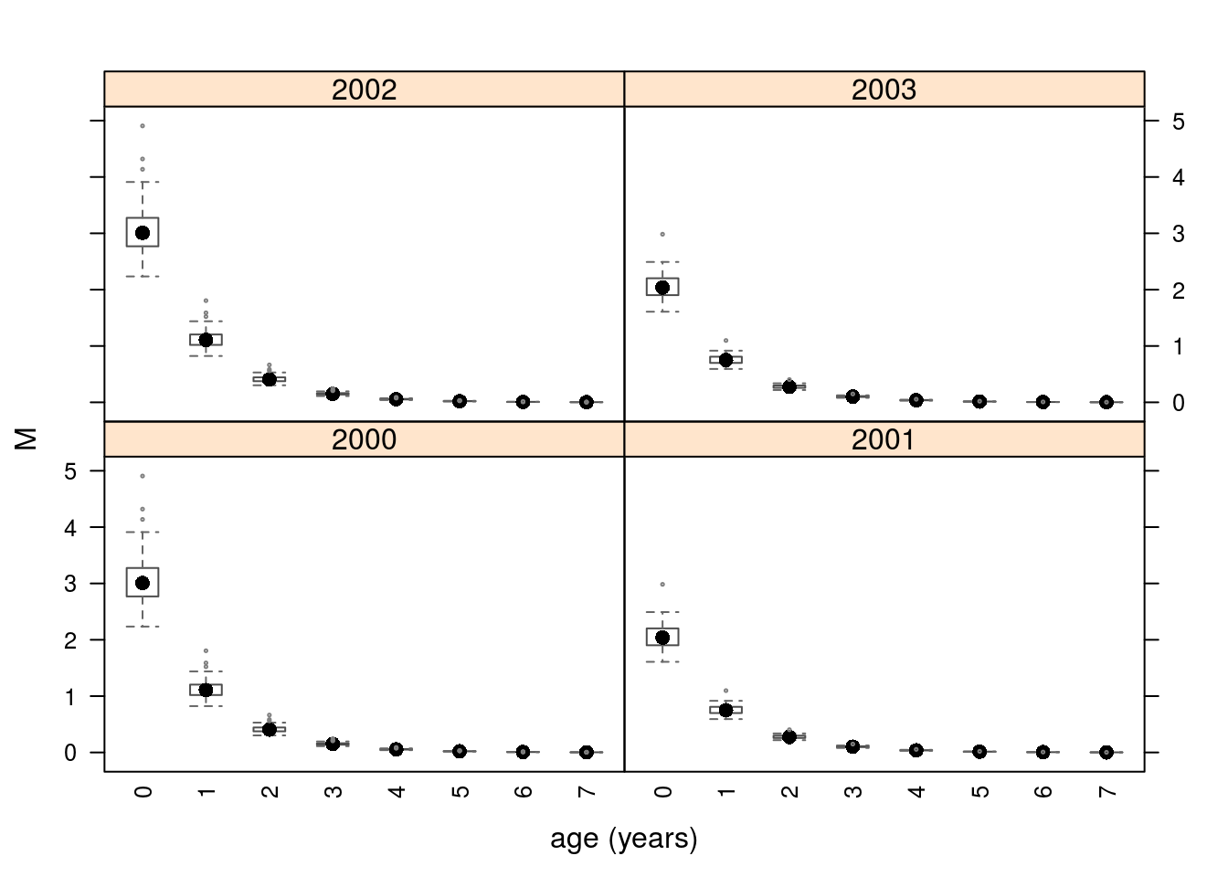
Natural mortality with age and year trend.
References
Ernesto Jardim, Colin P. Millar, Iago Mosqueira, Finlay Scott, Giacomo Chato Osio, Marco Ferretti, Nekane Alzorriz, Alessandro Orio; What if stock assessment is as simple as a linear model? The a4a initiative. ICES J Mar Sci 2015; 72 (1): 232-236. doi: icesjms/fsu050
Kenchington, T. J. (2014), Natural mortality estimators for information-limited fisheries. Fish Fish, 15: 533-562. doi: 10.1111/faf.12027.
Colin P. Millar, Ernesto Jardim, Finlay Scott, Giacomo Chato Osio, Iago Mosqueira, Nekane Alzorriz; Model averaging to streamline the stock assessment process. ICES J Mar Sci 2015; 72 (1): 93-98. doi: icesjms/fsu043
Scott F, Jardim E, Millar CP, Cervino S (2016) An Applied Framework for Incorporating Multiple Sources of Uncertainty in Fisheries Stock Assessments. PLoS ONE 11(5): e0154922. doi: 10.1371/journal.pone.0154922
More information
Documentation can be found at (http://flr-project.org/FLa4a). You are welcome to:
- Submit suggestions and bug-reports at: (https://github.com/flr/FLa4a/issues)
- Send a pull request on: (https://github.com/flr/FLa4a/)
- Compose a friendly e-mail to the maintainer, see
packageDescription('FLa4a')
Software Versions
- R version 3.4.1 (2017-06-30)
- FLCore: 2.6.5
- FLa4a: 1.1.3
- Compiled: Mon Sep 18 15:20:09 2017
License
This document is licensed under the Creative Commons Attribution-ShareAlike 4.0 International license.