Short term forecasts help projecting the stock to forecast the implications of different management choices over a limited number of years. There are three necessary ingredients when projecting in FLR:

a stock object that you will forecast and about which you have made some assumptions regarding what will happen in the future,
a stock-recruitment relationship,
a projection control specifying what the targets are and when to hit them.

In FLR, the method for short term forecasts is called fwd(), which takes an FLStock, FLSR, and fwdControl.

Required packages

To follow this tutorial you should have installed the following packages:

CRAN: ggplot2
FLR: FLCore, FLash, FLAssess, FLBRP, ggplotFL

if you are using Windows, please use the 32-bit R version

You can do so as follows,

install.packages(c("FLAssess","FLBRP","ggplotFL"), repos="http://flr-project.org/R")

The example used here is for the ple4 data that is available in FLR. This needs to be loaded first.

# Load the required packages
library(FLAssess)
library(FLash)
library(ggplotFL)
library(FLBRP)
# Load the data
data(ple4)
summary(ple4)

An object of class "FLStock"

Name: Plaice in IV 
Description: Imported from a VPA file. ( N:\Projecten\ICES WG\Demersale werkgroep  [...] 
Quant: age 
Dims:  age  year    unit    season  area    iter
    10  52  1   1   1   1   

Range:  min max pgroup  minyear maxyear minfbar maxfbar 
    1   10  10  1957    2008    2   6   

catch         : [ 1 52 1 1 1 1 ], units =  t 
catch.n       : [ 10 52 1 1 1 1 ], units =  10^3 
catch.wt      : [ 10 52 1 1 1 1 ], units =  kg 
discards      : [ 1 52 1 1 1 1 ], units =  t 
discards.n    : [ 10 52 1 1 1 1 ], units =  10^3 
discards.wt   : [ 10 52 1 1 1 1 ], units =  kg 
landings      : [ 1 52 1 1 1 1 ], units =  t 
landings.n    : [ 10 52 1 1 1 1 ], units =  10^3 
landings.wt   : [ 10 52 1 1 1 1 ], units =  kg 
stock         : [ 1 52 1 1 1 1 ], units =  t 
stock.n       : [ 10 52 1 1 1 1 ], units =  10^3 
stock.wt      : [ 10 52 1 1 1 1 ], units =  kg 
m             : [ 10 52 1 1 1 1 ], units =  m 
mat           : [ 10 52 1 1 1 1 ], units =   
harvest       : [ 10 52 1 1 1 1 ], units =  f 
harvest.spwn  : [ 10 52 1 1 1 1 ], units =   
m.spwn        : [ 10 52 1 1 1 1 ], units =

Extending the stock object for the projections

Our ple4 stock goes up to 2008, and in this example we want to make a 3-year projection, so we need to extend the stock by 3 years (nyears).

The projection will predict abundances in the future, but what will the future stock weights, maturity, natural mortality, etc. be like? The assumptions about these will affect the outcome of the projection. Rather than using window() or trim() that make all future data NA, we use the stf() function (short term forecast) that has several options that allow one to control the assumptions about the future stock parameters.

These assumptions specify how many years you want to average over to set future values. For example, wts.nyears is the number of years over which to calculate the *.wt, *.spwn, mat and m slots. By default this is set to 3 years. This is a fairly standard assumption for short term forecasts, i.e. the future weights at age will be the same as the average of the last 3 years. This assumes that what is going to happen in the next few years will be similar to what happened in the last few years.

A simple 3-year forecast for the weights, natural mortality, etc., assuming these are equal to their averages over the last 3 years, is done by:

maxyr_stk <- range(ple4)[["maxyear"]]
ple4_stf <- stf(ple4,nyears=3,wts.nyears=3, na.rm=TRUE)
maxyr_stf <- range(ple4_stf)[["maxyear"]]

Previously, the stock went up to 2008. Now the stock goes up to 2011 and the future weights are equal to the average of the last three observed years, as can be observed from the last six years of the stock weights of the ple4_stf object.

range(ple4_stf)

      min       max plusgroup   minyear   maxyear   minfbar   maxfbar 
        1        10        10      1957      2011         2         6

stock.wt(ple4_stf)[,ac((maxyr_stf-5):maxyr_stf)]

An object of class "FLQuant"
An object of class "FLQuant"
, , unit = unique, season = all, area = unique

    year
age  2006     2007     2008     2009     2010     2011    
  1  0.053000 0.048000 0.050000 0.050333 0.050333 0.050333
  2  0.129000 0.093000 0.114000 0.112000 0.112000 0.112000
  3  0.195000 0.239000 0.200000 0.211333 0.211333 0.211333
  4  0.321000 0.241000 0.278000 0.280000 0.280000 0.280000
  5  0.354000 0.337000 0.355000 0.348667 0.348667 0.348667
  6  0.424000 0.394000 0.429000 0.415667 0.415667 0.415667
  7  0.439000 0.458000 0.484000 0.460333 0.460333 0.460333
  8  0.506000 0.412000 0.627000 0.515000 0.515000 0.515000
  9  0.583000 0.526000 0.598000 0.569000 0.569000 0.569000
  10 0.730673 0.548489 0.730672 0.669945 0.669945 0.669945

units:  kg

For maturity the same assumption (of the future being the same as the average of the last 3 years) holds, but those maturities were assumed constant already.

mat(ple4_stf)[,ac((maxyr_stf-5):maxyr_stf)]

An object of class "FLQuant"
An object of class "FLQuant"
, , unit = unique, season = all, area = unique

    year
age  2006 2007 2008 2009 2010 2011
  1  0.0  0.0  0.0  0.0  0.0  0.0 
  2  0.5  0.5  0.5  0.5  0.5  0.5 
  3  0.5  0.5  0.5  0.5  0.5  0.5 
  4  1.0  1.0  1.0  1.0  1.0  1.0 
  5  1.0  1.0  1.0  1.0  1.0  1.0 
  6  1.0  1.0  1.0  1.0  1.0  1.0 
  7  1.0  1.0  1.0  1.0  1.0  1.0 
  8  1.0  1.0  1.0  1.0  1.0  1.0 
  9  1.0  1.0  1.0  1.0  1.0  1.0 
  10 1.0  1.0  1.0  1.0  1.0  1.0 

units:

Notice that the future fishing mortality has also been set (average of the last 3 years, by default).

ggplot(harvest(ple4_stf)[,ac((maxyr_stf-5):maxyr_stf)]) + geom_line(aes(x=age, y=data)) + facet_wrap(~year)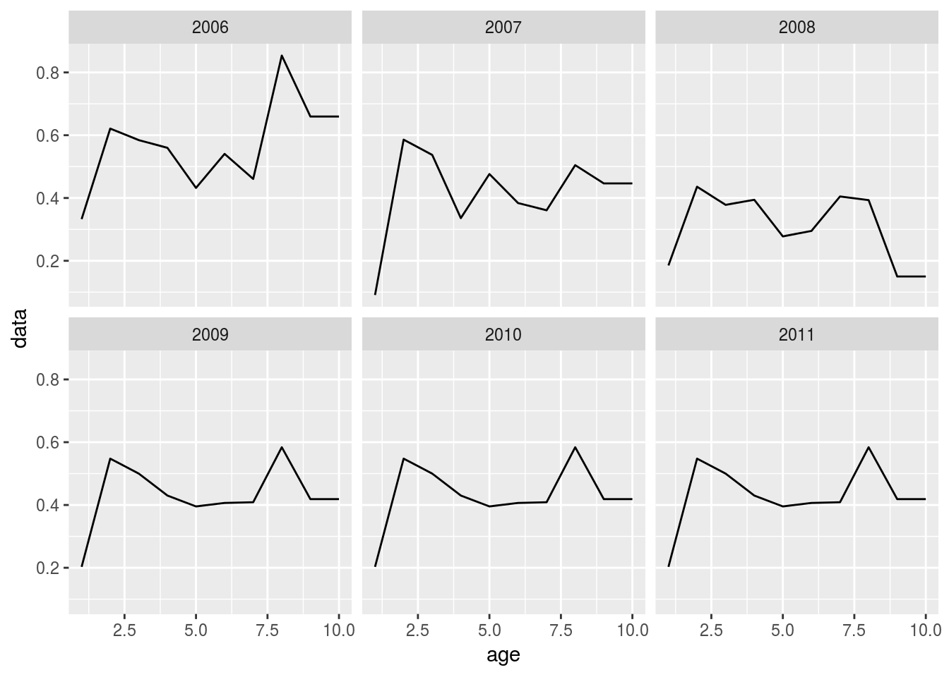

The stock numbers at age and the catch numbers at age are not forecast yet - this is what the fwd() function will perform later.

stock.n(ple4_stf)[,ac((maxyr_stf-5):maxyr_stf)]

An object of class "FLQuant"
An object of class "FLQuant"
, , unit = unique, season = all, area = unique

    year
age  2006     2007     2008     2009     2010     2011    
  1  820006.3 949341.2 844041.2       NA       NA       NA
  2  554592.5 531914.3 784234.7       NA       NA       NA
  3  422068.8 269655.1 267892.4       NA       NA       NA
  4   88052.9 212889.2 142573.0       NA       NA       NA
  5  136368.1  45514.9 137660.4       NA       NA       NA
  6   17534.5  80086.2  25575.8       NA       NA       NA
  7   16289.7   9240.6  49356.8       NA       NA       NA
  8    4114.0   9297.5   5828.1       NA       NA       NA
  9    2688.5   1585.1   5078.7       NA       NA       NA
  10   2854.5   3660.1   6750.3       NA       NA       NA

units:  10^3

Meanwhile, the landings and discards are average forecast ratios (proportion of total catch) of what is discarded and what is landed over the last 3 years of data.

discards.n(ple4_stf)[,ac((maxyr_stf-5):maxyr_stf)]

An object of class "FLQuant"
An object of class "FLQuant"
, , unit = unique, season = all, area = unique

    year
age  2006       2007       2008       2009       2010       2011      
  1  2.2047e+05 7.7312e+04 1.3541e+05 9.9308e-01 9.9308e-01 9.9308e-01
  2  2.2508e+05 2.0514e+05 2.5263e+05 9.3166e-01 9.3166e-01 9.3166e-01
  3  1.1022e+05 6.9312e+04 3.7393e+04 5.7876e-01 5.7876e-01 5.7876e-01
  4  1.0656e+04 1.0735e+04 6.2370e+03 2.0786e-01 2.0786e-01 2.0786e-01
  5  3.0000e+03 1.4370e+03 2.2820e+03 7.5111e-02 7.5111e-02 7.5111e-02
  6  4.1000e+02 7.1510e+03 5.1700e+02 1.4546e-01 1.4546e-01 1.4546e-01
  7  7.5400e+02 2.0400e+02 8.8820e+03 2.5884e-01 2.5884e-01 2.5884e-01
  8  1.9400e+02 1.6490e+03 8.9100e+02 3.5033e-01 3.5033e-01 3.5033e-01
  9  0.0000e+00 0.0000e+00 0.0000e+00 0.0000e+00 0.0000e+00 0.0000e+00
  10 0.0000e+00 0.0000e+00 0.0000e+00 0.0000e+00 0.0000e+00 0.0000e+00

units:  10^3

landings.n(ple4_stf)[,ac((maxyr_stf-5):maxyr_stf)]

An object of class "FLQuant"
An object of class "FLQuant"
, , unit = unique, season = all, area = unique

    year
age  2006       2007       2008       2009       2010       2011      
  1  3.5500e+02 1.2860e+03 3.8000e+02 6.9226e-03 6.9226e-03 6.9226e-03
  2  1.8987e+04 1.9205e+04 1.0970e+04 6.8339e-02 6.8339e-02 6.8339e-02
  3  6.7465e+04 3.7309e+04 4.2865e+04 4.2124e-01 4.2124e-01 4.2124e-01
  4  2.5254e+04 4.7053e+04 3.7970e+04 7.9214e-01 7.9214e-01 7.9214e-01
  5  4.2525e+04 1.4971e+04 2.9476e+04 9.2489e-01 9.2489e-01 9.2489e-01
  6  6.5550e+03 1.7142e+04 5.7000e+03 8.5454e-01 8.5454e-01 8.5454e-01
  7  4.9670e+03 2.4590e+03 6.7520e+03 7.4116e-01 7.4116e-01 7.4116e-01
  8  2.0530e+03 1.8560e+03 9.1200e+02 6.4967e-01 6.4967e-01 6.4967e-01
  9  1.2350e+03 5.4300e+02 6.7300e+02 1.0000e+00 1.0000e+00 1.0000e+00
  10 1.3190e+03 1.2590e+03 8.9600e+02 1.0000e+00 1.0000e+00 1.0000e+00

units:  10^3

# Compare above landings.n for the forecast years with
yearMeans((landings.n(ple4)/(landings.n(ple4)+discards.n(ple4)))[,ac((maxyr_stk-2):maxyr_stk)])

An object of class "FLQuant"
An object of class "FLQuant"
, , unit = unique, season = all, area = unique

    year
age  1        
  1  0.0069226
  2  0.0683387
  3  0.4212371
  4  0.7921356
  5  0.9248890
  6  0.8545368
  7  0.7411596
  8  0.6496718
  9  1.0000000
  10 1.0000000

units:  NA

# Furthermore, landings and discards proportions sum to 1
landings.n(ple4_stf)[,ac((maxyr_stf-2):maxyr_stf)] + discards.n(ple4_stf)[,ac((maxyr_stf-2):maxyr_stf)]

An object of class "FLQuant"
An object of class "FLQuant"
, , unit = unique, season = all, area = unique

    year
age  2009 2010 2011
  1  1    1    1   
  2  1    1    1   
  3  1    1    1   
  4  1    1    1   
  5  1    1    1   
  6  1    1    1   
  7  1    1    1   
  8  1    1    1   
  9  1    1    1   
  10 1    1    1   

units:  1000

The stock-recruitment relationship (SRR)

A short term forecast does not use an SRR (in the traditional sense). Instead, it generally assumes that recruitment in the future is some mean (e.g. geometric mean) of the historic recruitments. However, we still need to have an SRR that contains this mean value, which is what we mimic for this example. First, we estimate the geometic mean recruitment, that we then add to an SRR object

mean_rec <- exp(mean(log(rec(ple4))))
ple4_sr <- as.FLSR(ple4, model="geomean")
params(ple4_sr)['a',] <- mean_rec
params(ple4_sr)

An object of class "FLPar"
params
    a 
9e+05 
units:  NA

The control object

The final thing we need to set up is the control object. This tells the projection what to do, i.e. what level of fishing mortality to use.

A standard scenario for a short term forecast is the ‘status quo’ scenario, assuming that the future mean fishing mortality will be the same as the mean of the last X years (X depending on the stock). We will set up this scenario as a simple example using the Fbar in the last year (2008), being 0.356 per year.

round(fbar(ple4),3)

An object of class "FLQuant"
, , unit = unique, season = all, area = unique

     year
age   1957  1958  1959  1960  1961 
  all 0.269 0.321 0.367 0.368 0.348

      [ ...  42 years]

     year
age   2004  2005  2006  2007  2008 
  all 0.640 0.623 0.548 0.464 0.356

ggplot(fbar(ple4), aes(x=year,y=data)) + geom_line()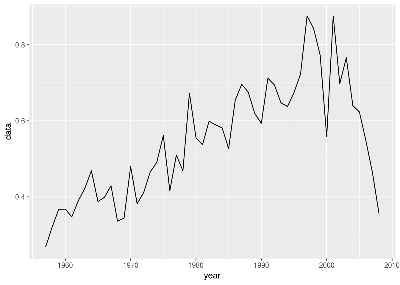

Below, we define the last year of the stock and the status quo Fbar fbar_SQ.

fbar_SQ <- mean(fbar(ple4)[,as.character(maxyr_stk)])

Now we introduce the control object: fwdControl(). This takes 1 argument - a data.frame that sets:

The quantity (or type) of the target (we are using Fbar but can also set catch etc. - see medium term forecast tutorial)
The value of the target, here status quo F
The year the target is to be hit
Some other things that we will ignore for now

Let’s make the data.frame

# Set the control object - year, quantity and value for the moment
ctrl_target <- data.frame(year = 2009:2011, quantity = "f", val = fbar_SQ)
ctrl_f <- fwdControl(ctrl_target)
ctrl_f


Target
  year quantity min    val max
1 2009        f  NA 0.3563  NA
2 2010        f  NA 0.3563  NA
3 2011        f  NA 0.3563  NA

   
    min     val     max    
  1      NA 0.35631      NA
  2      NA 0.35631      NA
  3      NA 0.35631      NA

We see that we have what looks like our ctrl_target, but now it has two more columns (min and max). There is another table underneath which is for uncertainty, but that we ignore here for the short term forecast examples.

Running the STF

Below we run a simple short term forecast (STF) with ‘status quo’ future fishing mortality. Remember we had to make assumptions about the future (weights, fishing mortality pattern, discard ratio, etc.).

This is done using fwd(), which takes three objects: the stock, the control object, the SRR. It returns an updated FLStock object. This update has forecast stock numbers, based on the recruitment, fishing mortality, and natural mortality assumptions. Because we now have stock numbers, we can calculate forecast ssb.

ple4_sq <- fwd(ple4_stf, ctrl = ctrl_f, sr = ple4_sr)

Below, we check if the recruitment in the forecast stock indeed corresponds to the mean recruitment

mean_rec

[1] 900370

rec(ple4_sq)[,ac((maxyr_stf-5):maxyr_stf)]

An object of class "FLQuant"
An object of class "FLQuant"
, , unit = unique, season = all, area = unique

   year
age 2006   2007   2008   2009   2010   2011  
  1 820006 949341 844041 900370 900370 900370

units:  NA

Similarly, we check if the fbar in the forecast stock indeed corresponds to status quo fishing mortality.

round(fbar_SQ,3)

[1] 0.356

round(fbar(ple4_sq)[,ac((maxyr_stf-5):maxyr_stf)],3)

An object of class "FLQuant"
An object of class "FLQuant"
, , unit = unique, season = all, area = unique

     year
age   2006  2007  2008  2009  2010  2011 
  all 0.548 0.464 0.356 0.356 0.356 0.356

units:  f

The stock numbers are calculated using the recruitment and future mortality assumptions.

stock.n(ple4_sq)[,ac((maxyr_stf-5):maxyr_stf)]

An object of class "FLQuant"
An object of class "FLQuant"
, , unit = unique, season = all, area = unique

    year
age  2006     2007     2008     2009     2010     2011    
  1  820006.3 949341.2 844041.2 900369.9 900369.9 900369.9
  2  554592.5 531914.3 784234.7 634556.4 695149.1 695149.1
  3  422068.8 269655.1 267892.4 458861.8 374263.6 410001.4
  4   88052.9 212889.2 142573.0 166055.3 280909.2 229119.3
  5  136368.1  45514.9 137660.4  86954.4 107361.5 181619.3
  6   17534.5  80086.2  25575.8  94351.2  57762.5  71318.6
  7   16289.7   9240.6  49356.8  17228.2  62135.0  38039.5
  8    4114.0   9297.5   5828.1  29788.4  11325.1  40844.9
  9    2688.5   1585.1   5078.7   3558.4  17078.0   6492.8
  10   2854.5   3660.1   6750.3   9212.2   8330.8  16575.1

units:  NA

Note that the future harvest slot is different from the harvest from the one we set up, but that the selection pattern is the same: F at age has been multiplied by a constant value to give us the target Fbar value.

round(harvest(ple4_stf)[,ac((maxyr_stf-2):maxyr_stf)],3)

An object of class "FLQuant"
An object of class "FLQuant"
, , unit = unique, season = all, area = unique

    year
age  2009  2010  2011 
  1  0.203 0.203 0.203
  2  0.548 0.548 0.548
  3  0.500 0.500 0.500
  4  0.430 0.430 0.430
  5  0.395 0.395 0.395
  6  0.407 0.407 0.407
  7  0.409 0.409 0.409
  8  0.584 0.584 0.584
  9  0.419 0.419 0.419
  10 0.419 0.419 0.419

units:  f

round(harvest(ple4_sq)[,ac((maxyr_stf-2):maxyr_stf)],3)

An object of class "FLQuant"
An object of class "FLQuant"
, , unit = unique, season = all, area = unique

    year
age  2009  2010  2011 
  1  0.159 0.159 0.159
  2  0.428 0.428 0.428
  3  0.391 0.391 0.391
  4  0.336 0.336 0.336
  5  0.309 0.309 0.309
  6  0.318 0.318 0.318
  7  0.320 0.320 0.320
  8  0.456 0.456 0.456
  9  0.327 0.327 0.327
  10 0.327 0.327 0.327

units:  f

harvest(ple4_stf)[,ac((maxyr_stf-2):maxyr_stf)] / harvest(ple4_sq)[,ac((maxyr_stf-2):maxyr_stf)]

An object of class "FLQuant"
An object of class "FLQuant"
, , unit = unique, season = all, area = unique

    year
age  2009   2010   2011  
  1  1.2797 1.2797 1.2797
  2  1.2797 1.2797 1.2797
  3  1.2797 1.2797 1.2797
  4  1.2797 1.2797 1.2797
  5  1.2797 1.2797 1.2797
  6  1.2797 1.2797 1.2797
  7  1.2797 1.2797 1.2797
  8  1.2797 1.2797 1.2797
  9  1.2797 1.2797 1.2797
  10 1.2797 1.2797 1.2797

units:  NA

The catch numbers come from the predicted abundance and harvest rates using the Baranov equation. The catches are then split into landings and discards using the average ratios computed by stf().

landings.n(ple4_sq)[,ac((maxyr_stf-5):maxyr_stf)]

An object of class "FLQuant"
An object of class "FLQuant"
, , unit = unique, season = all, area = unique

    year
age  2006     2007     2008     2009     2010     2011    
  1    355.00  1286.00   380.00   871.47   871.47   871.47
  2  18987.00 19205.00 10970.00 14418.91 15795.74 15795.74
  3  67465.00 37309.00 42865.00 59684.58 48680.81 53329.26
  4  25254.00 47053.00 37970.00 35832.72 60616.80 49441.17
  5  42525.00 14971.00 29476.00 20398.74 25186.06 42606.28
  6   6555.00 17142.00  5700.00 20939.33 12819.21 15827.72
  7   4967.00  2459.00  6752.00  3332.27 12018.13  7357.58
  8   2053.00  1856.00   912.00  6773.26  2575.09  9287.29
  9   1235.00   543.00   673.00   947.53  4547.50  1728.89
  10  1319.00  1259.00   896.00  2453.01  2218.31  4413.60

units:  NA

discards.n(ple4_sq)[,ac((maxyr_stf-5):maxyr_stf)]

An object of class "FLQuant"
An object of class "FLQuant"
, , unit = unique, season = all, area = unique

    year
age  2006     2007     2008     2009     2010     2011    
  1  220473.0  77312.0 135406.0 125015.3 125015.3 125015.3
  2  225077.0 205140.0 252629.0 196572.8 215343.2 215343.2
  3  110215.0  69312.0  37393.0  82004.2  66885.5  73272.3
  4   10656.0  10735.0   6237.0   9402.9  15906.5  12973.9
  5    3000.0   1437.0   2282.0   1656.6   2045.4   3460.1
  6     410.0   7151.0    517.0   3564.4   2182.1   2694.3
  7     754.0    204.0   8882.0   1163.8   4197.2   2569.5
  8     194.0   1649.0    891.0   3652.4   1388.6   5008.1
  9       0.0      0.0      0.0      0.0      0.0      0.0
  10      0.0      0.0      0.0      0.0      0.0      0.0

units:  NA

We can see the projection using a plot here

plot(ple4_sq) + geom_vline(lty=2,xintercept=an(ISOdate(maxyr_stk+1,1,1)))

Short term forecast with many F scenarios

Typically when running STF you explore several different future F scenarios. The scenarios are based on ‘F status quo’, which we calculated above as the mean F of the last X years.

For a 3 year STF the F pattern is:

year 1: fbar_status_quo
year 2: fbar_status_quo * fbar_multiplier
year 3: fbar_status_quo * fbar_multiplier

Note that year 1 is typically called the ‘intermediate year’ (in ICES, this would be the year the Expert Group meets to run the assessment, and status quo F for the intermediate year is a common assumption), and the fbar_multiplier is the same for years 2 and 3

We are going to run several STFs with different values for the fbar_multiplier

fbar_multiplier <- seq(from = 0, to = 2, by = 0.2)

Next we are going to build a data.frame that creates these scenarios. Each column in the dataframe is a year, each row is a scenario. Note that if you project for more than 3 years you will need to add more columns / years to the matrix

fbar_scenarios <- cbind(rep(fbar_SQ,length(fbar_multiplier)),
                        fbar_multiplier*fbar_SQ,
                        fbar_multiplier*fbar_SQ)

Another scenario we are interested in is \(F_{0.1}\). We can calculate this using FLBRP (or maybe you already have a value).

f01 <- c(refpts(brp(FLBRP(ple4)))["f0.1","harvest"])
# Add the F0.1 scenario as a final scenario 
fbar_scenarios <- rbind(fbar_scenarios, c(fbar_SQ,f01,f01))

# Add some names
colnames(fbar_scenarios) <- c("2009","2010","2011")
rownames(fbar_scenarios) <- c(fbar_multiplier, "f01")
fbar_scenarios

	2009	2010	2011
0	0.3563	0.0000	0.0000
0.2	0.3563	0.0713	0.0713
0.4	0.3563	0.1425	0.1425
0.6	0.3563	0.2138	0.2138
0.8	0.3563	0.2850	0.2850
1	0.3563	0.3563	0.3563
1.2	0.3563	0.4276	0.4276
1.4	0.3563	0.4988	0.4988
1.6	0.3563	0.5701	0.5701
1.8	0.3563	0.6414	0.6414
2	0.3563	0.7126	0.7126
f01	0.3563	0.0876	0.0876

There are various results we want to extract from the STF, like predicted Catch, SSB and the relative change in these. First, make an empty matrix in which to store the results.

stf_results <- matrix(NA,nrow = nrow(fbar_scenarios),ncol = 8)
# Set some column names
colnames(stf_results) <- c('Fbar',
    paste0('Catch',maxyr_stk+1), 
    paste0('Catch',maxyr_stk+2),
    paste0('Catch',maxyr_stk+3),
    paste0('SSB',maxyr_stk+2),
    paste0('SSB',maxyr_stk+3),
    paste0('SSB_change_',maxyr_stk+2,'-',maxyr_stk+3,'(%)'),
    paste0('Catch_change_',maxyr_stk,'-',maxyr_stk+2,'(%)'))

# Set up an FLStocks object to store the resulting FLStock each time
stk_stf <- FLStocks()
# Loop over the scenarios (each row in the fbar_scenarios table)
for (scenario in 1:nrow(fbar_scenarios)) {
    cat("Scenario: ", scenario, "\n")
    flush.console()
    # Make a target object with F values for that scenario
    # Set the control object - year, quantity and value for the moment
    ctrl_target <- data.frame(year = (maxyr_stf-2):maxyr_stf,
                              quantity = "f",
                              val = fbar_scenarios[scenario,])
    # ctrl_target
    ctrl_f <- fwdControl(ctrl_target)
    # Run the forward projection. We could include an additional argument, maxF.
    # By default the value of maxF is 2.0. It could be increased to 10.0, say,
    # so that F is less limited, and the bound is not hit (not a problem here).
    ple4_fwd <- fwd(ple4_stf, ctrl = ctrl_f, sr = ple4_sr)#, maxF = 10.0)
    ## Check it has worked - uncomment out to check scenario by scenario
    # plot(ple4_fwd[,ac(2001:2011)])
    # Store the result - if you want to, comment out if unnecessary
    stk_stf[[as.character(scenario)]] <- ple4_fwd

    # Fill results table
    stf_results[scenario,1] <- round(fbar(ple4_fwd)[,ac(2011)],3) # final stf year
    stf_results[scenario,2] <- catch(ple4_fwd)[,ac(maxyr_stk+1)] # 1st stf year
    stf_results[scenario,3] <- catch(ple4_fwd)[,ac(maxyr_stk+2)] # 2nd stf year
    stf_results[scenario,4] <- catch(ple4_fwd)[,ac(maxyr_stk+3)] # final stf year
    stf_results[scenario,5] <- ssb(ple4_fwd)[,ac(maxyr_stk+2)] # 2nd stf year
    stf_results[scenario,6] <- ssb(ple4_fwd)[,ac(maxyr_stk+3)] # final stf year
    
    # change in ssb in last two stf years
    stf_results[scenario,7] <- round((ssb(ple4_fwd)[,ac(maxyr_stk+3)]-ssb(ple4_fwd)[,ac(maxyr_stk+2)])/
                                      ssb(ple4_fwd)[,ac(maxyr_stk+2)]*100,1) 
    
    # change in catch from true year, to 2nd to last stf year
    stf_results[scenario,8] <- round((catch(ple4_fwd)[,ac(maxyr_stk+2)]-catch(ple4_fwd)[,ac(maxyr_stk)])/
                                      catch(ple4_fwd)[,ac(maxyr_stk)]*100,1) 
}
# Give the FLStocks object some names
names(stk_stf) <- rownames(fbar_scenarios)

# Plotting
plot(stk_stf)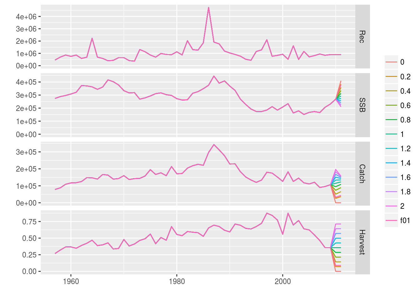

The different scenarios are plotted above. The table of results is given below.

stf_results

Fbar	Catch2009	Catch2010	Catch2011	SSB2010	SSB2011	SSB_change_2010-2011(%)	Catch_change_2008-2010(%)
0.000	106368	0	0	268307	410158	52.9	-100.0
0.071	106368	26377	36153	268307	383213	42.8	-72.5
0.143	106368	50963	65598	268307	358124	33.5	-46.9
0.214	106368	73885	89367	268307	334758	24.8	-23.1
0.285	106368	95259	108345	268307	312995	16.7	-0.8
0.356	106368	115195	123285	268307	292719	9.1	19.9
0.428	106368	133794	134831	268307	273827	2.1	39.3
0.499	106368	151151	143535	268307	256221	-4.5	57.4
0.570	106368	167352	149864	268307	239810	-10.6	74.3
0.641	106368	182478	154218	268307	224511	-16.3	90.0
0.713	106368	196604	156937	268307	210245	-21.6	104.7
0.088	106368	32168	43457	268307	377302	40.6	-66.5

More information

You can submit bug reports, questions or suggestions on this tutorial at https://github.com/flr/doc/issues.
Or send a pull request to https://github.com/flr/doc/
For more information on the FLR Project for Quantitative Fisheries Science in R, visit the FLR webpage, http://flr-project.org.

Software Versions

R version 3.4.1 (2017-06-30)
FLCore: 2.6.5
FLAssess: 2.6.1
FLash: 2.5.8
ggplotFL: 2.6.1
ggplot2: 2.2.1
FLBRP: 2.5.2
Compiled: Mon Sep 18 09:24:48 2017

License

This document is licensed under the Creative Commons Attribution-ShareAlike 4.0 International license.

Author information

Jan-Jaap Poos Wageningen UR. Wageningen Marine Research. Haringkade 1, IJmuiden, The Netherlands.

Katell Hamon Wageningen UR. Wageningen Economic Research. Alexanderveld 5, The Hague, The Netherlands.

Short Term Forecasting for advice using FLash

18 September, 2017