Required packages

To follow this tutorial you should have installed the following packages:

• CRAN: ggplot2
• FLR: FLCore, FLash,FLXSA,FLBRP, ggplotFL

You can do so as follows,

install.packages(c("ggplot2"))
install.packages(c("FLa4a","FLash","FLXSA","FLBRP","ggplotFL"), repos="http://flr-project.org/R")

# Loads all necessary packages
library(FLa4a)
library(FLash)
library(FLXSA)
library(FLBRP)
library(ggplotFL)

CONDITIONING THE OPERATING MODEL

Conditioning the operating model is a key step in building an MSE analysis, as it allows operating models to be considered “plausible” in the sense that they are consistent with observed data. In this tutorial, the a4a assessment model is fitted to the data within the ple4 FLStock and ple4.index FLIndex objects to produce stk, the operating model FLStock object. An mcmc method within the a4a assessment is used to obtain parameter uncertainty, reflected in the iter dimension of stk.

Read in stock assessment data

data(ple4)
data(ple4.index)
stk <- ple4
idx <- FLIndices(idx=ple4.index)

Set up the iteration and projection window parameters

In this tutorial, 20 iterations are used along with a 12-year projection window. A 3-year period is used for to calculate averages needed for projections (e.g. mean weights, etc.).

it <- 20    # iterations
y0 <- range(stk)["minyear"] # initial data year
dy <- range(stk)["maxyear"] # final data year
iy <- dy+1  # initial year of projection (also intermediate year)
ny <- 12    # number of years to project from intial year
fy <- dy+ny # final year
nsqy <- 3   # number of years to compute status quo metrics

Fit stock assessment model a4a

Set up the operating model (including parameter uncertainty) based on fitting the a4a assessment model to data. Reference points are obtained for a “median” stk (stk0) to mimic best estimates of reference points used in the ICES MSY approach.

# Set up the catchability submodel with a smoothing spline
# (setting up a 'list' allows for more than one index)
qmod <- list(~s(age, k=6))
# Set up the fishing mortality submodel as a tensor spline,
# which allows age and year to interact
fmod <- ~te(replace(age, age>9,9), year, k=c(6,8))
# Set up the MCMC parameters
mcsave <- 100
mcmc <- it * mcsave
# Fit the model
fit <- sca(stk, idx, fmodel = fmod, qmodel = qmod, fit = "MCMC", 
       mcmc = SCAMCMC(mcmc = mcmc, mcsave = mcsave, mcprobe = 0.4))
# Update the FLStock object
stk <- stk + fit
# Reduce to keep one iteration only for reference points
stk0 <- qapply(stk, iterMedians)

Fit stock-recruit model

A Beverton-Holt stock-recruit model is fitted for each iteration, with residuals generated for the projection window based on the residuals from the historic period. A stock-recruit model is also fitted to the “median” stk for reference points.

# Fit the stock-recruit model
srbh <- fmle(as.FLSR(stk, model="bevholt"), method="L-BFGS-B", 
        lower=c(1e-6, 1e-6), upper=c(max(rec(stk)) * 3, Inf))
srbh0 <- fmle(as.FLSR(stk0, model="bevholt"), method="L-BFGS-B", 
         lower=c(1e-6, 1e-6), upper=c(max(rec(stk)) * 3, Inf))
# Generate stock-recruit residuals for the projection period
srbh.res <- rnorm(it, FLQuant(0, dimnames=list(year=iy:fy)), mean(c(apply(residuals(srbh), 6, sd))))

Calculate reference points and set up the operating model for the projection window

Reference points based on the “median” stk, assuming (for illustrative purposes only) that Bpa=0.5Bmsy and Blim=Bpa/1.4. The stf method is applied to the operating model stk object in order to have the necessary data (mean weights, etc.) for the projection window.

# Calculate the reference points
brp <- brp(FLBRP(stk0, srbh0))
Fmsy <- c(refpts(brp)["msy","harvest"])
msy <- c(refpts(brp)["msy","yield"])
Bmsy <- c(refpts(brp)["msy","ssb"])
Bpa <- 0.5*Bmsy
Blim <- Bpa/1.4
# Prepare the FLStock object for projections
stk <- stf(stk, fy-dy, nsqy, nsqy)

SET UP OBSERVATION ERROR MODEL ELEMENTS

Estimate the index catchabilities from the a4a fit (without simulation)

Observation error is introduced through the index catchability-at-age

# Set up the FLIndices object and populate it
# (note, FLIndices potentially has more than one index, hence the for loop)
idcs <- FLIndices()
for (i in 1:length(idx)){
#   Set up FLQuants and calculate mean and sd for catchability
    lst <- mcf(list(index(idx[[i]]), stock.n(stk0))) # make FLQuants same dimensions
    idx.lq <- log(lst[[1]]/lst[[2]]) # log catchability of index
    idx.qmu <- idx.qsig <- stock.n(iter(stk,1)) # create quants
    idx.qmu[] <- yearMeans(idx.lq) # allocate same mean-at-age to every year
    idx.qsig[] <- sqrt(yearVars(idx.lq)) # allocate same sd-at-age to every year
#   Build index catchability based on lognormal distribution with mean and sd calculated above
    idx.q <- rlnorm(it, idx.qmu, idx.qsig)
    idx_temp <- idx.q * stock.n(stk)
    idx_temp <- FLIndex(index=idx_temp, index.q=idx.q) # generate initial index
    range(idx_temp)[c("startf", "endf")] <- c(0, 0) # timing of index (as proportion of year)
    idcs[[i]] <- idx_temp
}
names(idcs) <- names(idx)
idx<-idcs[1]

SET UP MSE LOOP

o <- function(stk, idx, assessmentYear, dataYears) {
    # dataYears is a position vector, not the years themselves
    stk.tmp <- stk[, dataYears]
    # add small amount to avoid zeros
    catch.n(stk.tmp) <- catch.n(stk.tmp) + 0.1
    # Generate the indices - just data years
    idx.tmp <- lapply(idx, function(x) x[,dataYears])
  # Generate observed index
    for (i in 1:length(idx)) index(idx[[i]])[, assessmentYear] <- 
    stock.n(stk)[, assessmentYear]*index.q(idx[[i]])[, assessmentYear]
  list(stk=stk.tmp, idx=idx.tmp, idx.om=idx)
}

xsa <- function(stk, idx){
  # Set up XSA settings
    control  <- FLXSA.control(tol = 1e-09, maxit=99, min.nse=0.3, fse=2.0,
                              rage = -1, qage = range(stk)["max"]-1, shk.n = TRUE, shk.f = TRUE,
                              shk.yrs = 5, shk.ages= 5, window = 100, tsrange = 99, tspower = 0)
  # Fit XSA
  fit <- FLXSA(stk, idx, control)
  # convergence diagnostic (quick and dirty)
  maxit <- c("maxit" = fit@control@maxit)
  # Update stk
  stk   <- transform(stk, harvest = harvest(fit), stock.n = stock.n(fit))
  return(list(stk = stk, converge = maxit))
}

getCtrl <- function(values, quantity, years, it){
    dnms <- list(iter=1:it, year=years, c("min", "val", "max"))
    arr0 <- array(NA, dimnames=dnms, dim=unlist(lapply(dnms, length)))
    arr0[,,"val"] <- unlist(values)
    arr0 <- aperm(arr0, c(2,3,1))
    ctrl <- fwdControl(data.frame(year=years, quantity=quantity, val=NA))
    ctrl@trgtArray <- arr0
    ctrl
}

vy <- ac(iy:fy)
TAC <- FLQuant(NA, dimnames=list(TAC="all", year=c(dy,vy), iter=1:it))
TAC[,ac(dy)] <- catch(stk)[,ac(dy)]
TAC[,ac(iy)] <- TAC[,ac(dy)] #assume same TAC in the first intermediate year
ctrl <- getCtrl(c(TAC[,ac(iy)]), "catch", iy, it)
# Set up the operating model FLStock object
stk.om <- fwd(stk, control=ctrl, sr=srbh, sr.residuals = exp(srbh.res), sr.residuals.mult = TRUE)

set.seed(231) # set seed to ensure comparability between different runs
for(i in vy[-length(vy)]){
  # set up simulations parameters
    ay <- an(i)
    cat(i, " > ")
  flush.console()
    vy0 <- 1:(ay-y0) # data years (positions vector) - one less than current year
    sqy <- (ay-y0-nsqy+1):(ay-y0) # status quo years (positions vector) - one less than current year

  # apply observation error
    oem <- o(stk.om, idx, i, vy0)
    stk.mp <- oem$stk
    idx.mp <- oem$idx
    idx <- oem$idx.om

  # perform assessment
  out.assess <- xsa(stk.mp, idx.mp)
  stk.mp <- out.assess$stk
  
  # apply ICES MSY-like Rule to obtain Ftrgt
  # (note this is not the ICES MSY rule, but is similar)
  flag <- ssb(stk.mp)[,ac(ay-1)]<Bpa
  Ftrgt <- ifelse(flag,ssb(stk.mp)[,ac(ay-1)]*Fmsy/Bpa,Fmsy) 

  # project the perceived stock to get the TAC for ay+1
  fsq.mp <- yearMeans(fbar(stk.mp)[,sqy]) # Use status quo years defined above
  ctrl <- getCtrl(c(fsq.mp, Ftrgt), "f", c(ay, ay+1), it)
  stk.mp <- stf(stk.mp, 2)
  gmean_rec <- c(exp(yearMeans(log(rec(stk.mp)))))
  stk.mp <- fwd(stk.mp, control=ctrl, sr=list(model="mean", params = FLPar(gmean_rec,iter=it)))
  TAC[,ac(ay+1)] <- catch(stk.mp)[,ac(ay+1)]

  # apply the TAC to the operating model stock
  ctrl <- getCtrl(c(TAC[,ac(ay+1)]), "catch", ay+1, it)
  stk.om <- fwd(stk.om, control=ctrl,sr=srbh, sr.residuals = exp(srbh.res), sr.residuals.mult = TRUE)
}

PERFORMANCE STATISTICS

#Some example performance statstics, but first isolate the projection period
stk.tmp<-window(stk.om,start=iy)
# annual probability of being below Blim
(risky<-iterSums(ssb(stk.tmp)/Blim<1)/it)

, , unit = unique, season = all, area = unique

     year
age   2018 2019 2020 2021 2022
  all 1.00 1.00 1.00 0.85 0.15

      [ ...  2 years]

     year
age   2025 2026 2027 2028 2029
  all 0    0    0    0    0   

# mean probabiity of being below Blim in the first half of the projection period
mean(risky[,1:trunc(length(risky)/2)])

[1] 0.6667

# ...and second half
mean(risky[,(trunc(length(risky)/2)+1):length(risky)])

[1] 0

# plot of SSB relative to Bmsy
boxplot(data~year,data=as.data.frame(ssb(stk.tmp)),main="SSB")
abline(h=Bmsy,col="red")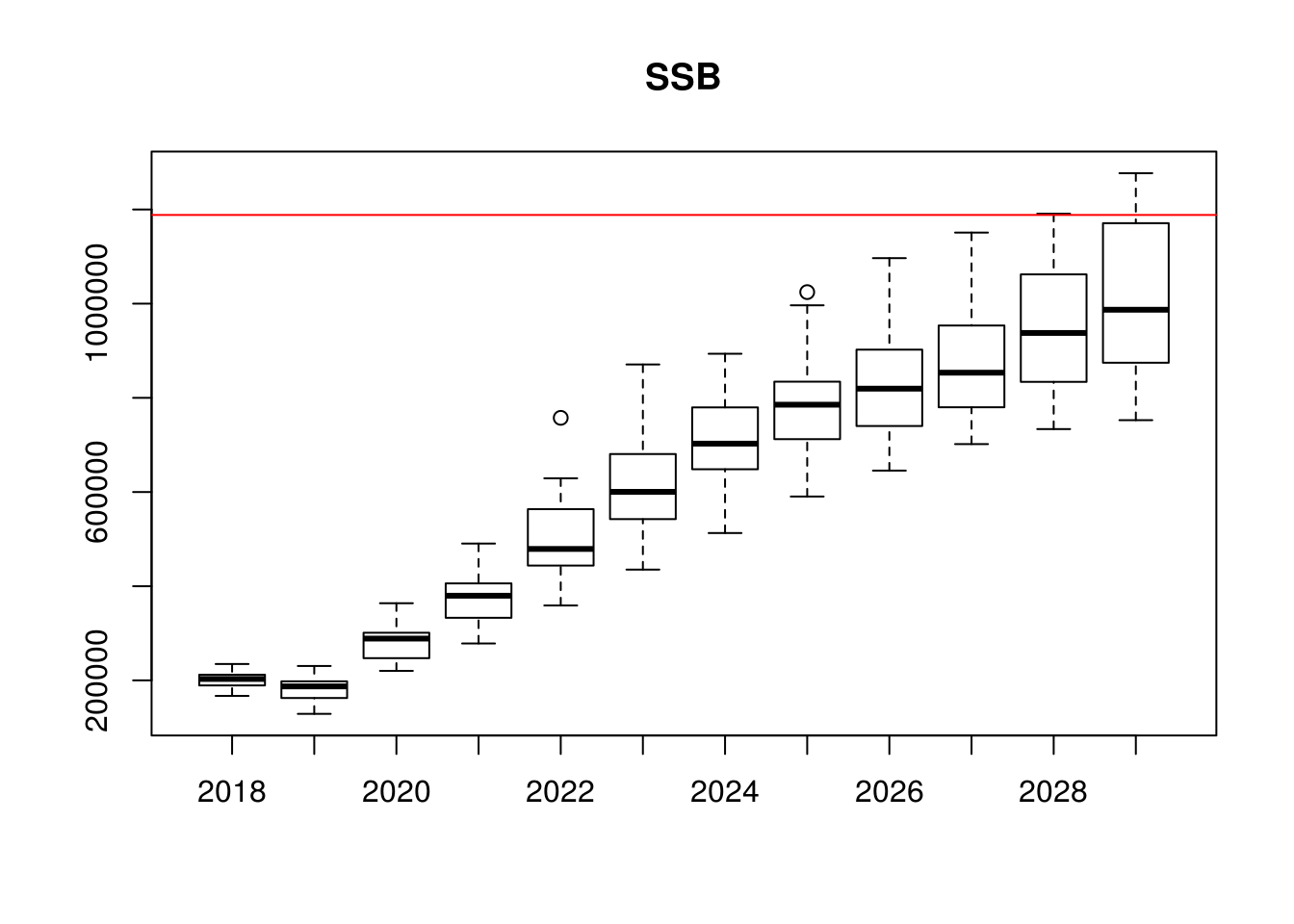

# plot of landings relative to MSY yield
boxplot(data~year,data=as.data.frame(landings(stk.tmp)),main="Landings")
abline(h=msy,col="red")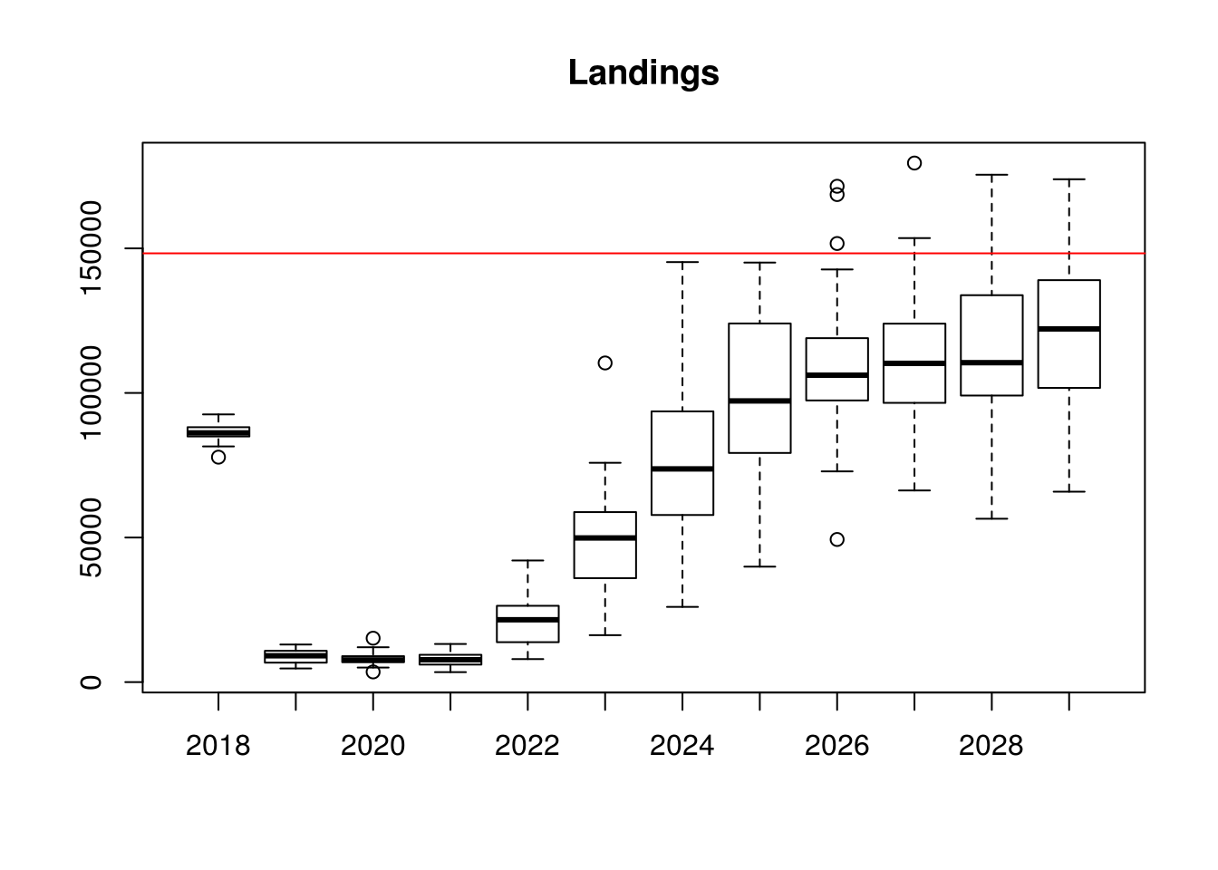

plot(FLStocks(stk.om=stk.om, stk.mp=stk.mp)) + theme(legend.position="top") + geom_vline(aes(xintercept=2009))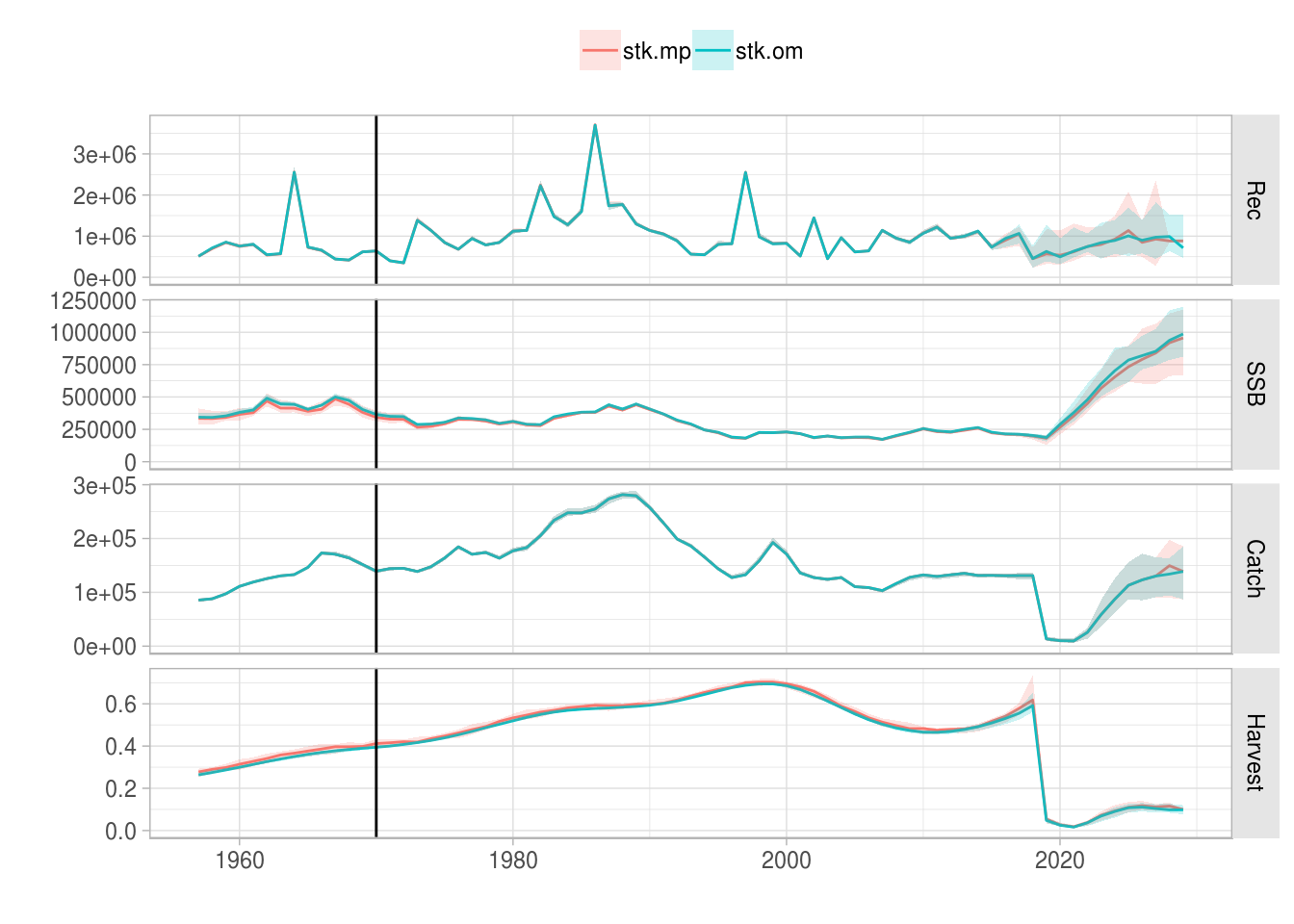

Results for applying an ICES MSY-like rule, comparing the operating model to the management procedure

References

Punt, A.E., Butterworth, D.S., de Moor, C.L., De Oliveira, J.A.A. and M. Haddon (2016). Management Strategy Evaluation: Best Practices. Fish and Fisheries, 17(2): 303-334. DOI: 10.1111/faf.12104.

More information

• You can submit bug reports, questions or suggestions on this tutorial at https://github.com/flr/doc/issues.
• Or send a pull request to https://github.com/flr/doc/
• For more information on the FLR Project for Quantitative Fisheries Science in R, visit the FLR webpage, http://flr-project.org.