Getting started with bbm package.
Leire Ibaibarriaga & Sonia Sanchez
30 August, 2022
bbm_manual.RmdIntroduction
bbm is an open-source R package that provides an FLR implementation of the two-stage biomass-based model for the Bay of Biscay anchovy (Ibaibarriaga et al. 2008). This model describes the stock dynamics in terms of biomass and separates the population into two stages: recruits and adults. Thus, it has lower data demands than fully age-structured models, while it is able to track the main dynamics of the population with more detail than biomass dynamic models. Besides the application to the Bay of Biscay anchovy, similar models have been applied to other case studies (Giannoulaki et al. 2014; Gras et al. 2014; Roel and Butterworth 2000; Roel, Oliveira, and Beggs 2009).
The implementation available in this package estimates the model parameters by maximum likelihood through the TMB package (Kristensen et al. 2016). Additionally, the model has been generalised for an unlimited number of indices that can occur at different times of the year. The package uses the S4 classes and methods developed by the FLR project (http://flr-project.org/R; Kell et al. 2007).
This document explains the basic use of the package bbm. The package and documentation are available at http://flr-project.org/bbm.
Installation
The package requires the packages TMB and FLCore to be installed. TMB can be installed from CRAN using the install.packages() command, whereas FLCore can be installed from the FLR project repository:
  install.packages('TMB')
  install.packages(c("FLCore"), repos="http://flr-project.org/R")
An stable version of bbm can be installed from the FLR repository (http://flr-project.org/R) with the command:
install.packages(c("bbm"), repos="http://flr-project.org/R")A development version is available from GitHub repository (https://github.com/flr/bbm/).
    library(devtools)
    install_github('flr/bbm')
Once installed, the package can be loaded using:
library(bbm)Getting started: Bay of Biscay anchovy
The package contains data and additional objects required to run the Bay of Biscay anchovy example from Ibaibarriaga et al. (2008). They can be loaded using:
data(ane)The dataset documentation can be consulted by using:
?aneThe data consist on four objects: catch.ane, indicesB.ane, indicesP.ane, control.ane and inits.ane. The first object, catch.ane, is an FLQuant with the Bay of Biscay anchovy catch in tonnes from 1987 to 2006 for the two age classes (recruits and adults) and two periods (before and after the spring surveys in mid-May). Note that the catch of the second period of the last year were not available in Ibaibarriaga et al. (2008). However, the model fitting function does not allow any missing value in the catch.ane object, and the NA’s were replaced by very small non-negative values so that the total catch was 0.001 and the age 1 proportion was 0.5.
  class(catch.ane)
#> [1] "FLQuant"
#> attr(,"package")
#> [1] "FLCore"
  dim(catch.ane)
#> [1]  2 20  1  2  1  1
  catch.ane
#> An object of class "FLQuant"
#> , , unit = unique, season = 1, area = unique
#>
#>    year
#> age 1987       1988       1989       1990       1991       1992
#>   1  2711.0000  2602.0000  1723.0000  9314.0000  3903.0000 11933.0000
#>   2  5607.0000  1262.0000  2153.0000  1259.0000  6288.0000  4433.0000
#>    year
#> age 1993       1994       1995       1996       1997       1998
#>   1  6414.0000  3795.0000  5718.0000  4570.0000  4323.0000  5898.0000
#>   2  7763.0000  9807.0000  8832.0000  4676.0000  2912.0000  2090.0000
#>    year
#> age 1999       2000       2001       2002       2003       2004
#>   1  2067.0000  6298.0000  5481.0000  1962.0000   625.0000  2754.0000
#>   2  8828.0000  5712.0000  5987.0000  5776.0000  1754.0000  1869.0000
#>    year
#> age 2005       2006
#>   1   102.0000   287.0000
#>   2   688.0000   311.0000
#>
#> , , unit = unique, season = 2, area = unique
#>
#>    year
#> age 1987       1988       1989       1990       1991       1992
#>   1  3960.0000  8554.0000  2039.0000 20249.0000  5048.0000 17565.0000
#>   2  2583.0000  2400.0000  2403.0000  3325.0000  3148.0000  3461.0000
#>    year
#> age 1993       1994       1995       1996       1997       1998
#>   1 17812.0000 12425.0000  9560.0000 17869.0000 11450.0000 17841.0000
#>   2  7619.0000  7725.0000  5255.0000  5964.0000  1806.0000  5747.0000
#>    year
#> age 1999       2000       2001       2002       2003       2004
#>   1  7753.0000 16957.0000 17911.0000  4367.0000  3848.0000  9211.0000
#>   2  7758.0000  7925.0000 10760.0000  5387.0000  4253.0000  2446.0000
#>    year
#> age 2005       2006
#>   1    81.0000     0.0005
#>   2   291.0000     0.0005
#>
#> units:  NA
The catch in tonnes per age class and period can be plotted as:
xyplot(data~year|age+season, data=catch.ane, type="l", main="Total Catch (t)")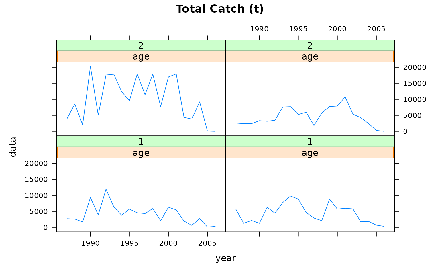
Let’s define nyrs as the number of years:
Then, we can plot the proportion of the recruits (age 1) in the catch for each of the periods:
  xyplot( data~year|season,
          data=FLQuants(period1=catch.ane[1,,,1,,]/quantSums(catch.ane[,,,1,,]),
                        period2=catch.ane[1,1:(nyrs-1),,2,,]/quantSums(catch.ane[,1:(nyrs-1),,2,,])),
          type="l", main="Catch proportion of recruits by period", ylab="")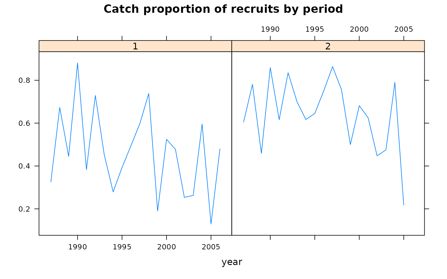
The object indicesB.ane is of class FLIndices, which is a list of two elements of the FLIndex class. Each of them contains the data of the two spring surveys: BIOMAN DEPM survey conducted by AZTI and the PELGAS acoustic survey conducted by IFREMER. The index slot of each FLIndex object contains the total biomass estimates at the time of each survey.
  length(indicesB.ane)
#> [1] 2
  names(indicesB.ane)
#> [1] "depm"     "acoustic"
  lapply(indicesB.ane, index)
#> $ depm
#> An object of class "FLQuant"
#> , , unit = unique, season = all, area = unique
#>
#>      year
#> age   1987   1988   1989   1990   1991   1992   1993   1994   1995   1996
#>   all  29365  63500  16720  97239  19276  90720     NA  60062  54700  39545
#>      year
#> age   1997   1998   1999   2000   2001   2002   2003   2004   2005   2006
#>   all  51176 101976  69074  44973 120403  30697  23962  19498   8002  21436
#>
#> units:  NA
#>
#> $ acoustic
#> An object of class "FLQuant"
#> , , unit = unique, season = all, area = unique
#>
#>      year
#> age   1987   1988   1989   1990   1991   1992   1993   1994   1995   1996
#>   all     NA     NA     NA     NA  64000  89000     NA  35000     NA     NA
#>      year
#> age   1997   1998   1999   2000   2001   2002   2003   2004   2005   2006
#>   all  63000  57000     NA  98484 137200  97051  29430  46018  15603  30649
#>
#> units:  NA
The object indicesP.ane is of class FLIndices, which is a list of two elements of the FLIndex class. Each of them contains the recruits proportion (in mass) estimates of the BIOMAN DEPM survey and the PELGAS acoustic survey.
  length(indicesP.ane)
#> [1] 2
  names(indicesP.ane)
#> [1] "depm"     "acoustic"
  lapply(indicesP.ane, index)
#> $ depm
#> An object of class "FLQuant"
#> , , unit = unique, season = all, area = unique
#>
#>      year
#> age   1987    1988    1989    1990    1991    1992    1993    1994    1995
#>   all 0.48476 0.83602 0.43553 0.93224 0.58472 0.94324      NA 0.57730 0.78439
#>      year
#> age   1996    1997    1998    1999    2000    2001    2002    2003    2004
#>   all      NA 0.75301 0.78800      NA      NA 0.57399 0.20693 0.69172 0.75131
#>      year
#> age   2005    2006
#>   all 0.25781 0.71282
#>
#> units:  NA
#>
#> $ acoustic
#> An object of class "FLQuant"
#> , , unit = unique, season = all, area = unique
#>
#>      year
#> age   1987    1988    1989    1990    1991    1992    1993    1994    1995
#>   all      NA      NA      NA      NA 0.44253 0.94875      NA      NA      NA
#>      year
#> age   1996    1997    1998    1999    2000    2001    2002    2003    2004
#>   all      NA 0.61108      NA      NA      NA 0.66274 0.18262 0.53456 0.80673
#>      year
#> age   2005    2006
#>   all 0.15414 0.54442
#>
#> units:  NA
Besides the index slot, it is important to specify the timing of each index within the range slot of each FLIndex. In this case, both surveys are assumed to occur simultaneously at mid-May, so the start and end dates of each survey (startf and endf) are set equal to 0.375 = 5.5/12.
  lapply(indicesB.ane, range)
#> $depm
#>       min       max plusgroup   minyear   maxyear    startf      endf
#>        NA        NA        NA  1987.000  2006.000     0.375     0.375
#>
#> $acoustic
#>       min       max plusgroup   minyear   maxyear    startf      endf
#>        NA        NA        NA  1987.000  2006.000     0.375     0.375
  lapply(indicesP.ane, range)
#> $depm
#>       min       max plusgroup   minyear   maxyear    startf      endf
#>        NA        NA        NA  1987.000  2006.000     0.375     0.375
#>
#> $acoustic
#>       min       max plusgroup   minyear   maxyear    startf      endf
#>        NA        NA        NA  1987.000  2006.000     0.375     0.375
Each survey is assumed to occur at the middle of the start and end dates. The fraction of the year until that date can be computed as:
  findicesB.ane <- unlist(lapply(indicesB.ane, function(x) return(mean(range(x)[c('startf','endf')]))))
  findicesB.ane
#>     depm acoustic
#>    0.375    0.375
  findicesP.ane <- unlist(lapply(indicesP.ane, function(x) return(mean(range(x)[c('startf','endf')]))))
  findicesP.ane
#>     depm acoustic
#>    0.375    0.375
The timing of the surveys is important as it will define the number of periods within the year. The function periods returns a list with the number of periods (nper), the fraction of the year corresponding to each period (f) and a vector indicating the beginning of which period corresponds to each index. In this case the timings of the biomass and recruits indices define two periods within the year, that correspond to 0.375 and 0.675 fractions. In addition, the two biomass indices provide information at the beginning of the second period and the two recruits proportion indices also.
  per <- periods(findicesB=findicesB.ane, findicesP=findicesP.ane)
  per
#> $nper
#> [1] 2
#>
#> $f
#> [1] 0.375 0.625
#>
#> $perindicesB
#>     depm acoustic
#>        2        2
#>
#> $perindicesP
#>     depm acoustic
#>        2        2
We can plot the total biomass from each index:
  dat <- FLQuants()
  for (i in 1:length(indicesB.ane)) dat[[i]] <- index(indicesB.ane[[i]])
  names(dat) <- names(indicesB.ane)
  xyplot( data~year|qname, data=dat,
          type="b", main="Total biomass by survey", ylab="Total biomass (t)")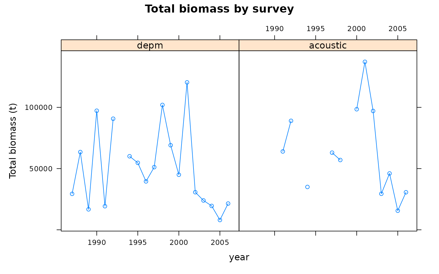
And the age 1 biomass proportion from each index:
  dat <- FLQuants()
  for (i in 1:length(indicesP.ane)) dat[[i]] <- index(indicesP.ane[[i]])
  names(dat) <- names(indicesP.ane)
  xyplot( data~year|qname, data=dat,
          type="b", main="Recruits' biomass proportion by survey", ylab="")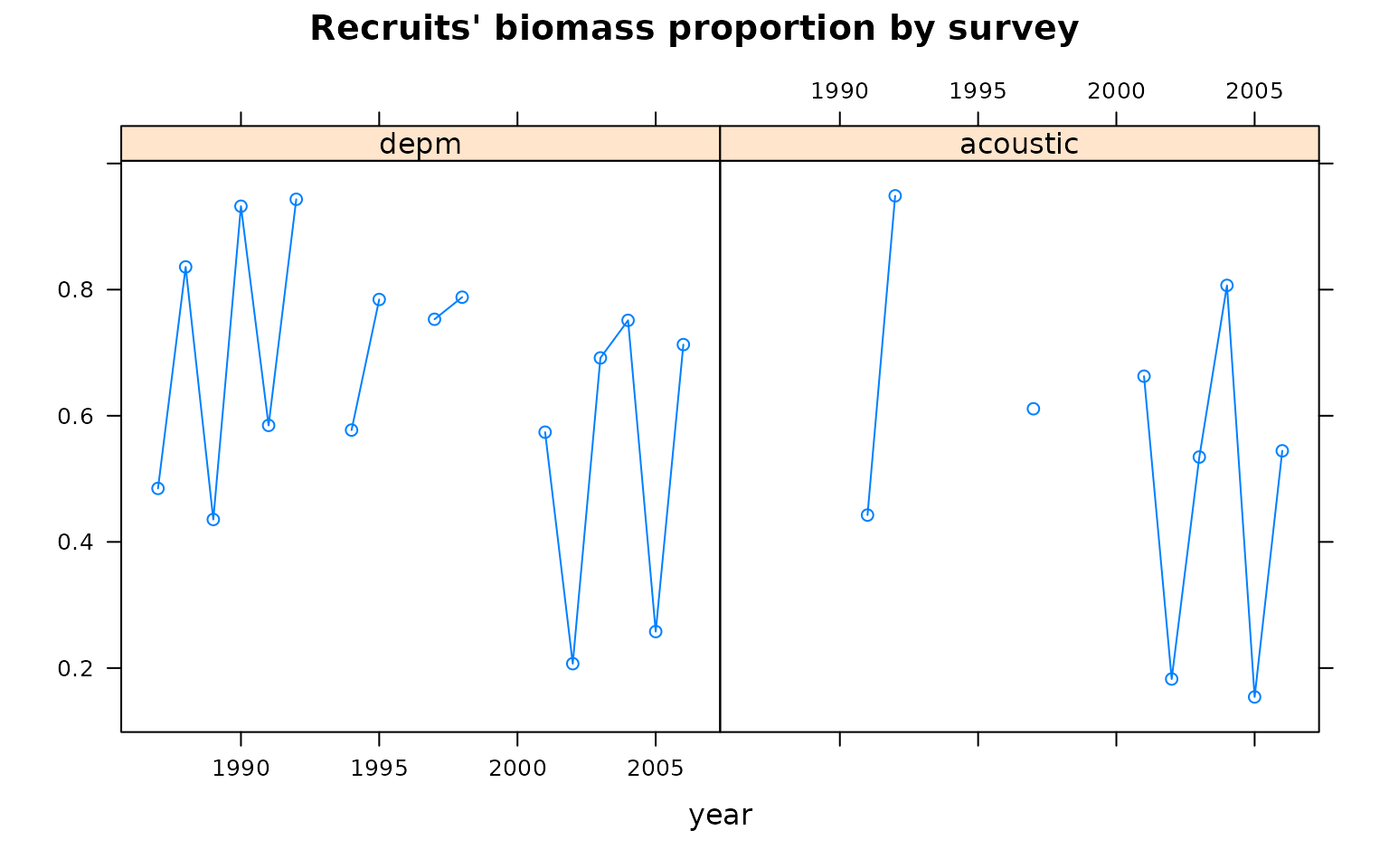
The control.ane object is of class bbmControl.
class(control.ane)
#> [1] "bbmControl"
#> attr(,"package")
#> [1] "bbm"
It has two slots: g and param.fix.
slotNames(control.ane)
#> [1] "g"         "param.fix"
The slot g is a named vector that specifies the instantaneous rate of biomass decrease for each age class, which is the difference between the annual intrinsic growth and the natural mortality rates. In Ibaibarriaga et al. (2008) the instantaneous biomass decrease was assumed to be age and time invariant and equal to 0.68.
control.ane@g
#>   rec adult
#>  0.68  0.68
The second slot of the control.ane object is param.fix that is of class FLPar for all the parameters to be estimated by the model.
class(control.ane@param.fix)
#> [1] "FLPar"
#> attr(,"package")
#> [1] "FLCore"
Each element of the param.fix slot takes the value 0 if the parameter has to be estimated and takes the value 1 if the parameter is fixed to the initial value. In this first example all the parameters are estimated. Other variants will be illustrated later.
control.ane@param.fix
#> An object of class "FLPar"
#> params
#>       q_depm   q_acoustic     psi_depm psi_acoustic      xi_depm  xi_acoustic
#>            0            0            0            0            0            0
#>           B0       R_1987       R_1988       R_1989       R_1990       R_1991
#>            0            0            0            0            0            0
#>       R_1992       R_1993       R_1994       R_1995       R_1996       R_1997
#>            0            0            0            0            0            0
#>       R_1998       R_1999       R_2000       R_2001       R_2002       R_2003
#>            0            0            0            0            0            0
#>       R_2004       R_2005       R_2006          mur         psir
#>            0            0            0            0            0
#> units:  NA NA NA NA NA NA NA NA NA NA NA NA NA NA NA NA NA NA NA NA NA NA NA NA NA NA NA NA NA
In other words, there are no fixed elements:
sum(control.ane@param.fix==1) # number of fixed parameters
#> [1] 0
The inits.ane object is of class FLPar and it contains initial values for all the model parameters.
class(inits.ane)
#> [1] "FLPar"
#> attr(,"package")
#> [1] "FLCore"
inits.ane
#> An object of class "FLPar"
#> params
#>       q_depm   q_acoustic     psi_depm psi_acoustic      xi_depm  xi_acoustic
#>            1            1           50           50            3            3
#>           B0       R_1987       R_1988       R_1989       R_1990       R_1991
#>        50000        80000        80000        80000        80000        80000
#>       R_1992       R_1993       R_1994       R_1995       R_1996       R_1997
#>        80000        80000        80000        80000        80000        80000
#>       R_1998       R_1999       R_2000       R_2001       R_2002       R_2003
#>        80000        80000        80000        80000        80000        80000
#>       R_2004       R_2005       R_2006          mur         psir
#>        80000        80000        80000           10            2
#> units:  NA NA NA NA NA NA NA NA NA NA NA NA NA NA NA NA NA NA NA NA NA NA NA NA NA NA NA NA NA
The initial parameters should provide biomasses large enough to support the level of observed catches. Given the instantaneous annual biomass decrease rates, the fraction of the year corresponding to each period, an FLQuant for the catches and an object of the class FLpar, the function calcPop calculates the resulting biomasses and checks that the resulting biomasses by age group are positive.
out <- calcPop(g=control.ane@g, f=per$f, catch=catch.ane, inits=inits.ane)
names(out)
#> [1] "stock.bio" "ok"
out$ok
#> [1] TRUE
out$stock.bio
#> An object of class "FLQuant"
#> , , unit = unique, season = 1, area = unique
#>
#>    year
#> age 1987  1988  1989  1990  1991  1992  1993  1994  1995  1996  1997  1998
#>   1 80000 80000 80000 80000 80000 80000 80000 80000 80000 80000 80000 80000
#>   2 50000 55783 57709 63943 47778 52243 40577 32365 32805 36797 34580 43166
#>    year
#> age 1999  2000  2001  2002  2003  2004  2005  2006
#>   1 80000 80000 80000 80000 80000 80000 80000 80000
#>   2 38728 41338 34441 28196 42474 54128 55866 68076
#>
#> , , unit = unique, season = 2, area = unique
#>
#>    year
#> age 1987  1988  1989  1990  1991  1992  1993  1994  1995  1996  1997  1998
#>   1 59607 59703 60477 53794 58558 51489 56347 58653 56960 57970 58188 56801
#>   2 33810 42116 42824 48443 31489 36581 24610 16447 17647 24398 24233 31610
#>    year
#> age 1999  2000  2001  2002  2003  2004  2005  2006
#>   1 60174 56449 57168 60266 61443 59569 61904 61741
#>   2 22240 27005 21419 16765 31370 40299 42686 52480
#>
#> units:  NA
Given catch.ane, indices.ane, control.ane and inits.ane, the model is fitted simply by:
  run <- bbm(catch.ane,
             indicesB=FLQuants(depm=index(indicesB.ane[[1]]), acoustic=index(indicesB.ane[[2]])),
             indicesP=FLQuants(depm=index(indicesP.ane[[1]]), acoustic=index(indicesP.ane[[2]])),
             findicesB=findicesB.ane,
             findicesP=findicesP.ane,
             control=control.ane, inits=inits.ane)
#> Constructing atomic D_lgamma
#> outer mgc:  2.991218
#> outer mgc:  2.983554
#> outer mgc:  2.994433
#> outer mgc:  2.980339
#> outer mgc:  2.989589
#> outer mgc:  2.985185
#> outer mgc:  2.990111
#> outer mgc:  2.984663
#> outer mgc:  2.986485
#> outer mgc:  2.988286
#> outer mgc:  2.987929
#> outer mgc:  2.986843
#> outer mgc:  2.987386
#> outer mgc:  2.987386
#> outer mgc:  2.987386
#> outer mgc:  2.987386
#> outer mgc:  2.987386
#> outer mgc:  2.987386
#> outer mgc:  2.987386
#> outer mgc:  2.987386
#> outer mgc:  2.987385
#> outer mgc:  2.987387
#> outer mgc:  2.987385
#> outer mgc:  2.987387
#> outer mgc:  2.987382
#> outer mgc:  2.98739
#> outer mgc:  2.987383
#> outer mgc:  2.987388
#> outer mgc:  2.98738
#> outer mgc:  2.987392
#> outer mgc:  2.987369
#> outer mgc:  2.987403
#> outer mgc:  2.987363
#> outer mgc:  2.987409
#> outer mgc:  2.987322
#> outer mgc:  2.98745
#> outer mgc:  2.98723
#> outer mgc:  2.987541
#> outer mgc:  2.987124
#> outer mgc:  2.987647
#> outer mgc:  2.986773
#> outer mgc:  2.987998
#> outer mgc:  2.986082
#> outer mgc:  2.988689
#> outer mgc:  2.986608
#> outer mgc:  2.988164
#> outer mgc:  3.008474
#> outer mgc:  2.96631
#> outer mgc:  2.986905
#> outer mgc:  2.987863
#> outer mgc:  2.986374
#> outer mgc:  2.988397
#> outer mgc:  2.986725
#> outer mgc:  2.988047
#> outer mgc:  2.9823
#> outer mgc:  2.992471
#> outer mgc:  2.985849
#> outer mgc:  2.988921
#> outer mgc:  2.987386
#> outer mgc:  2.991218
#> outer mgc:  2.983554
#> outer mgc:  2.994433
#> outer mgc:  2.980339
#> outer mgc:  2.989589
#> outer mgc:  2.985185
#> outer mgc:  2.990111
#> outer mgc:  2.984663
#> outer mgc:  2.986485
#> outer mgc:  2.988286
#> outer mgc:  2.987929
#> outer mgc:  2.986843
#> outer mgc:  2.987386
#> outer mgc:  2.987386
#> outer mgc:  2.987386
#> outer mgc:  2.987386
#> outer mgc:  2.987386
#> outer mgc:  2.987386
#> outer mgc:  2.987386
#> outer mgc:  2.987386
#> outer mgc:  2.987385
#> outer mgc:  2.987387
#> outer mgc:  2.987385
#> outer mgc:  2.987387
#> outer mgc:  2.987382
#> outer mgc:  2.98739
#> outer mgc:  2.987383
#> outer mgc:  2.987388
#> outer mgc:  2.98738
#> outer mgc:  2.987392
#> outer mgc:  2.987369
#> outer mgc:  2.987403
#> outer mgc:  2.987363
#> outer mgc:  2.987409
#> outer mgc:  2.987322
#> outer mgc:  2.98745
#> outer mgc:  2.98723
#> outer mgc:  2.987541
#> outer mgc:  2.987124
#> outer mgc:  2.987647
#> outer mgc:  2.986773
#> outer mgc:  2.987998
#> outer mgc:  2.986082
#> outer mgc:  2.988689
#> outer mgc:  2.986608
#> outer mgc:  2.988164
#> outer mgc:  3.008474
#> outer mgc:  2.96631
#> outer mgc:  2.986905
#> outer mgc:  2.987863
#> outer mgc:  2.986374
#> outer mgc:  2.988397
#> outer mgc:  2.986725
#> outer mgc:  2.988047
#> outer mgc:  2.9823
#> outer mgc:  2.992471
#> outer mgc:  2.985849
#> outer mgc:  2.988921
#> outer mgc:  282597.9
The output object is of class bbmFit.
  class(run)
#> [1] "bbmFit"
#> attr(,"package")
#> [1] "bbm"
And it has the following slots:
  slotNames(run)
#>  [1] "inputs"      "convergence" "message"     "fitSumm"     "params"
#>  [6] "params.se"   "vcov"        "stock.bio"   "indicesB"    "indicesP"
The convergence should be checked:
  run@convergence
#> [1] 0
The fitted model parameters and their corresponding standard errors can be extracted directly using the accessors:
  params(run)
#> An object of class "FLPar"
#> params
#>       q_depm   q_acoustic     psi_depm psi_acoustic      xi_depm  xi_acoustic
#>     2.64e-01     3.44e-01     3.90e+00     7.17e+00     2.24e+00     2.38e+00
#>           B0       R_1987       R_1988       R_1989       R_1990       R_1991
#>     6.55e+04     8.91e+04     1.27e+05     7.10e+04     1.69e+05     8.83e+04
#>       R_1992       R_1993       R_1994       R_1995       R_1996       R_1997
#>     2.83e+05     8.70e+04     1.01e+05     1.56e+05     1.05e+05     1.48e+05
#>       R_1998       R_1999       R_2000       R_2001       R_2002       R_2003
#>     1.82e+05     1.55e+05     1.83e+05     1.98e+05     5.98e+04     8.43e+04
#>       R_2004       R_2005       R_2006          mur         psir
#>     1.14e+05     3.61e+04     9.31e+04     1.16e+01     5.09e+00
#> units:  NA
  params.se(run)
#> An object of class "FLPar"
#> params
#>       q_depm   q_acoustic     psi_depm psi_acoustic      xi_depm  xi_acoustic
#>     3.82e-02     5.12e-02     1.43e+00     3.57e+00     2.72e-01     5.67e-01
#>           B0       R_1987       R_1988       R_1989       R_1990       R_1991
#>     2.56e+04     2.81e+03     3.39e+04          NaN     5.21e+04     1.30e+04
#>       R_1992       R_1993       R_1994       R_1995       R_1996       R_1997
#>     1.19e+05     2.38e+04     2.55e+04     6.37e+04     3.02e+04     4.19e+04
#>       R_1998       R_1999       R_2000       R_2001       R_2002       R_2003
#>     7.39e+04     6.88e+04     6.03e+04     5.24e+04          NaN          NaN
#>       R_2004       R_2005       R_2006          mur         psir
#>     2.85e+04          NaN     1.11e+04          NaN     1.99e+00
#> units:  NA
  vcov(run)
#> , , 1
#>
#>                    logq_depm logq_acoustic logpsi_depm logpsi_acoustic
#> logq_depm        0.020957252   0.007664286 -0.07639773    -0.055644319
#> logq_acoustic    0.007664286   0.022113190 -0.06971259    -0.058356490
#> logpsi_depm     -0.076397727  -0.069712587  0.13521670     0.015470203
#> logpsi_acoustic -0.055644319  -0.058356490  0.01547020     0.247261444
#> xi_depm         -0.093958781  -0.099275446 -0.04250018    -0.070744687
#> xi_acoustic     -0.142554296  -0.146216587 -0.02675519    -0.075436817
#> logB0            0.005807806   0.014334935  0.06944297     0.059293551
#> logR_1987        0.043823506   0.050461191  0.07535188     0.068811933
#> logR_1988       -0.007619600  -0.003262914  0.06732703     0.053285285
#> logR_1989        0.065236569   0.068932606  0.06043592     0.066764179
#> logR_1990       -0.035467860  -0.036230759  0.06251330     0.053733353
#> logR_1991        0.018938185   0.016923913  0.06272157     0.073226588
#> logR_1992       -0.077312929  -0.080237708  0.06665922     0.031036625
#> logR_1993        0.067735788   0.069213018  0.05047386     0.023555438
#> logR_1994        0.004080910   0.004307739  0.06967180     0.025041134
#> logR_1995       -0.048987939  -0.045666943  0.07586300     0.044614804
#> logR_1996        0.026073838   0.026626086  0.04682051     0.044048729
#> logR_1997       -0.017385516  -0.019422135  0.07834092     0.056123901
#> logR_1998       -0.050282010  -0.052188195  0.07882731     0.023991406
#> logR_1999       -0.022366019  -0.017839692  0.06378648     0.056764977
#> logR_2000       -0.012224509  -0.018591861  0.03418522     0.070661442
#> logR_2001       -0.021666320  -0.025123300  0.05627042     0.065352122
#> logR_2002        0.076959536   0.075089343  0.05975568     0.074319659
#> logR_2003        0.031807184   0.028168725  0.04589560     0.016350700
#> logR_2004       -0.001262388  -0.006134466  0.03148665    -0.004674095
#> logR_2005        0.116688536   0.114477326  0.04447625     0.018534233
#> logR_2006        0.028683333   0.025167750  0.05085288     0.021652400
#> mur              0.009409654   0.008871890  0.05907433     0.044152698
#> logpsir          0.194754560   0.196693406 -0.01626422    -0.010008751
#>                     xi_depm xi_acoustic        logB0     logR_1987    logR_1988
#> logq_depm       -0.09395878 -0.14255430  0.005807806  0.0438235058 -0.007619600
#> logq_acoustic   -0.09927545 -0.14621659  0.014334935  0.0504611906 -0.003262914
#> logpsi_depm     -0.04250018 -0.02675519  0.069442973  0.0753518814  0.067327030
#> logpsi_acoustic -0.07074469 -0.07543682  0.059293551  0.0688119333  0.053285285
#> xi_depm          0.07390166 -0.04201099  0.067337114  0.0696913629  0.078428157
#> xi_acoustic     -0.04201099  0.32118232  0.116128479  0.1284274286  0.114087282
#> logB0            0.06733711  0.11612848  0.153262059 -0.0394739361 -0.006849633
#> logR_1987        0.06969136  0.12842743 -0.039473936  0.0009938772 -0.038210219
#> logR_1988        0.07842816  0.11408728 -0.006849633 -0.0382102189  0.071576643
#> logR_1989        0.08460310  0.12209549 -0.064891476 -0.0987260482 -0.051211570
#> logR_1990        0.06891231  0.08361449  0.012689985 -0.0132813378  0.026036649
#> logR_1991        0.09054156  0.08770601 -0.032323822 -0.0653786776 -0.016900543
#> logR_1992        0.06868115  0.16132813  0.046650019  0.0179796427  0.062562406
#> logR_1993        0.07407151  0.07975942 -0.069627275 -0.0909559457 -0.060031457
#> logR_1994        0.08103983  0.11822797 -0.020875874 -0.0494878118 -0.007468251
#> logR_1995        0.07473276  0.12890012  0.022047892 -0.0080740425  0.037265540
#> logR_1996        0.05387489  0.09413956 -0.033119587 -0.0540669223 -0.024655763
#> logR_1997        0.08449539  0.12583016 -0.004523135 -0.0373761314  0.011245153
#> logR_1998        0.08851098  0.12813307  0.021345131 -0.0099455955  0.038527088
#> logR_1999        0.05994561  0.10017432  0.004058793 -0.0208462590  0.016178629
#> logR_2000        0.05329742  0.07761005 -0.001702424 -0.0238923569  0.008613997
#> logR_2001        0.06036118  0.11898887  0.003377632 -0.0227784139  0.015343114
#> logR_2002        0.10058334  0.08573877 -0.081580042 -0.1159707540 -0.067747705
#> logR_2003        0.11746987  0.13422141 -0.049175348 -0.0848356044 -0.031775832
#> logR_2004        0.10902656  0.19444034 -0.022331535 -0.0552492068 -0.005234377
#> logR_2005        0.14478519  0.11988966 -0.120827706 -0.1599571001 -0.103549456
#> logR_2006        0.12193066  0.13447253 -0.047159486 -0.0833212224 -0.028636914
#> mur              0.08429733  0.11687709 -0.024330182 -0.0507868522 -0.007521225
#> logpsir          0.06848135 -0.01728292 -0.164272879 -0.1674772853 -0.167102532
#>                   logR_1989    logR_1990    logR_1991   logR_1992   logR_1993
#> logq_depm        0.06523657 -0.035467860  0.018938185 -0.07731293  0.06773579
#> logq_acoustic    0.06893261 -0.036230759  0.016923913 -0.08023771  0.06921302
#> logpsi_depm      0.06043592  0.062513300  0.062721565  0.06665922  0.05047386
#> logpsi_acoustic  0.06676418  0.053733353  0.073226588  0.03103662  0.02355544
#> xi_depm          0.08460310  0.068912312  0.090541564  0.06868115  0.07407151
#> xi_acoustic      0.12209549  0.083614491  0.087706012  0.16132813  0.07975942
#> logB0           -0.06489148  0.012689985 -0.032323822  0.04665002 -0.06962728
#> logR_1987       -0.09872605 -0.013281338 -0.065378678  0.01797964 -0.09095595
#> logR_1988       -0.05121157  0.026036649 -0.016900543  0.06256241 -0.06003146
#> logR_1989       -0.03251213 -0.030554124 -0.079657913 -0.00176436 -0.10067066
#> logR_1990       -0.03055412  0.095645945  0.017960022  0.08577658 -0.04163747
#> logR_1991       -0.07965791  0.017960022  0.021738348  0.04470045 -0.08135101
#> logR_1992       -0.00176436  0.085776577  0.044700445  0.17731210 -0.03923294
#> logR_1993       -0.10067066 -0.041637467 -0.081351009 -0.03923294  0.07499174
#> logR_1994       -0.06605587  0.016127565 -0.029750353  0.04794345 -0.06432912
#> logR_1995       -0.02883913  0.060713506  0.015396512  0.10542621 -0.03641153
#> logR_1996       -0.06609205 -0.005989840 -0.041701417  0.01357802 -0.06429205
#> logR_1997       -0.05745195  0.039768263 -0.010306190  0.07954903 -0.05924819
#> logR_1998       -0.02971375  0.062875914  0.016784305  0.10794985 -0.03700232
#> logR_1999       -0.03804797  0.036892018 -0.002198503  0.06808998 -0.04402938
#> logR_2000       -0.03559990  0.029486558 -0.001381485  0.05353288 -0.04352667
#> logR_2001       -0.03949172  0.037889927 -0.001947956  0.07334805 -0.04763288
#> logR_2002       -0.12908112 -0.032612148 -0.085614081 -0.01556720 -0.10539396
#> logR_2003       -0.09806737 -0.001228359 -0.054183465  0.03419634 -0.08213535
#> logR_2004       -0.06894988  0.018591718 -0.031880133  0.06972287 -0.06333933
#> logR_2005       -0.16825700 -0.066395908 -0.126761185 -0.04634233 -0.12448016
#> logR_2006       -0.09690308  0.002551320 -0.051270430  0.03824531 -0.08121200
#> mur             -0.06598735  0.016818987 -0.028302483  0.04871177 -0.05965318
#> logpsir         -0.14918662 -0.158961113 -0.166697729 -0.19689254 -0.08120639
#>                    logR_1994    logR_1995    logR_1996     logR_1997
#> logq_depm        0.004080910 -0.048987939  0.026073838 -0.0173855162
#> logq_acoustic    0.004307739 -0.045666943  0.026626086 -0.0194221350
#> logpsi_depm      0.069671797  0.075862999  0.046820514  0.0783409171
#> logpsi_acoustic  0.025041134  0.044614804  0.044048729  0.0561239007
#> xi_depm          0.081039833  0.074732764  0.053874894  0.0844953943
#> xi_acoustic      0.118227974  0.128900120  0.094139563  0.1258301574
#> logB0           -0.020875874  0.022047892 -0.033119587 -0.0045231350
#> logR_1987       -0.049487812 -0.008074042 -0.054066922 -0.0373761314
#> logR_1988       -0.007468251  0.037265540 -0.024655763  0.0112451532
#> logR_1989       -0.066055868 -0.028839126 -0.066092052 -0.0574519452
#> logR_1990        0.016127565  0.060713506 -0.005989840  0.0397682630
#> logR_1991       -0.029750353  0.015396512 -0.041701417 -0.0103061901
#> logR_1992        0.047943453  0.105426210  0.013578021  0.0795490318
#> logR_1993       -0.064329120 -0.036411534 -0.064292052 -0.0592481938
#> logR_1994        0.063877977  0.031426448 -0.039303953  0.0024011180
#> logR_1995        0.031426448  0.167149423 -0.034842403  0.0535762430
#> logR_1996       -0.039303953 -0.034842403  0.082081803 -0.0151420159
#> logR_1997        0.002401118  0.053576243 -0.015142016  0.0805885369
#> logR_1998        0.030899609  0.080070730 -0.001868924  0.0544252249
#> logR_1999        0.005107669  0.046446574 -0.014895217  0.0200736540
#> logR_2000       -0.002147194  0.033300083 -0.014231346  0.0150393179
#> logR_2001        0.004979568  0.048267460 -0.011389069  0.0266809694
#> logR_2002       -0.074268805 -0.038746947 -0.073906162 -0.0655265890
#> logR_2003       -0.035264666  0.003861953 -0.050561755 -0.0244525383
#> logR_2004       -0.008126048  0.033008326 -0.029091709  0.0046943079
#> logR_2005       -0.101906885 -0.074730976 -0.100557011 -0.1055193636
#> logR_2006       -0.032849313  0.007941800 -0.049285185 -0.0209387319
#> mur             -0.015515475  0.024975936 -0.029887265 -0.0005302686
#> logpsir         -0.150261377 -0.190935930 -0.108884421 -0.1908252530
#>                    logR_1998    logR_1999     logR_2000    logR_2001
#> logq_depm       -0.050282010 -0.022366019 -0.0122245085 -0.021666320
#> logq_acoustic   -0.052188195 -0.017839692 -0.0185918605 -0.025123300
#> logpsi_depm      0.078827313  0.063786480  0.0341852220  0.056270423
#> logpsi_acoustic  0.023991406  0.056764977  0.0706614424  0.065352122
#> xi_depm          0.088510985  0.059945606  0.0532974160  0.060361176
#> xi_acoustic      0.128133074  0.100174321  0.0776100546  0.118988874
#> logB0            0.021345131  0.004058793 -0.0017024241  0.003377632
#> logR_1987       -0.009945596 -0.020846259 -0.0238923569 -0.022778414
#> logR_1988        0.038527088  0.016178629  0.0086139974  0.015343114
#> logR_1989       -0.029713750 -0.038047969 -0.0355998978 -0.039491716
#> logR_1990        0.062875914  0.036892018  0.0294865578  0.037889927
#> logR_1991        0.016784305 -0.002198503 -0.0013814852 -0.001947956
#> logR_1992        0.107949848  0.068089985  0.0535328820  0.073348045
#> logR_1993       -0.037002319 -0.044029376 -0.0435266659 -0.047632883
#> logR_1994        0.030899609  0.005107669 -0.0021471937  0.004979568
#> logR_1995        0.080070730  0.046446574  0.0333000834  0.048267460
#> logR_1996       -0.001868924 -0.014895217 -0.0142313458 -0.011389069
#> logR_1997        0.054425225  0.020073654  0.0150393179  0.026680969
#> logR_1998        0.165474142  0.030618719  0.0243272217  0.048372950
#> logR_1999        0.030618719  0.198289668 -0.0331683462  0.024405032
#> logR_2000        0.024327222 -0.033168346  0.1080934566  0.013487362
#> logR_2001        0.048372950  0.024405032  0.0134873622  0.070264069
#> logR_2002       -0.036946119 -0.046232533 -0.0378516979 -0.046191603
#> logR_2003        0.011033541 -0.016237495 -0.0150142558 -0.013372027
#> logR_2004        0.040199467  0.006311785  0.0030209418  0.012039418
#> logR_2005       -0.066833113 -0.081324731 -0.0709496851 -0.082662291
#> logR_2006        0.015215678 -0.013033741 -0.0133212121 -0.011622538
#> mur              0.027091758  0.007009931 -0.0002021729  0.004785408
#> logpsir         -0.186844253 -0.156394163 -0.1322482694 -0.162101376
#>                   logR_2002    logR_2003    logR_2004   logR_2005   logR_2006
#> logq_depm        0.07695954  0.031807184 -0.001262388  0.11668854  0.02868333
#> logq_acoustic    0.07508934  0.028168725 -0.006134466  0.11447733  0.02516775
#> logpsi_depm      0.05975568  0.045895599  0.031486650  0.04447625  0.05085288
#> logpsi_acoustic  0.07431966  0.016350700 -0.004674095  0.01853423  0.02165240
#> xi_depm          0.10058334  0.117469874  0.109026563  0.14478519  0.12193066
#> xi_acoustic      0.08573877  0.134221412  0.194440342  0.11988966  0.13447253
#> logB0           -0.08158004 -0.049175348 -0.022331535 -0.12082771 -0.04715949
#> logR_1987       -0.11597075 -0.084835604 -0.055249207 -0.15995710 -0.08332122
#> logR_1988       -0.06774770 -0.031775832 -0.005234377 -0.10354946 -0.02863691
#> logR_1989       -0.12908112 -0.098067365 -0.068949879 -0.16825700 -0.09690308
#> logR_1990       -0.03261215 -0.001228359  0.018591718 -0.06639591  0.00255132
#> logR_1991       -0.08561408 -0.054183465 -0.031880133 -0.12676118 -0.05127043
#> logR_1992       -0.01556720  0.034196344  0.069722865 -0.04634233  0.03824531
#> logR_1993       -0.10539396 -0.082135352 -0.063339332 -0.12448016 -0.08121200
#> logR_1994       -0.07426881 -0.035264666 -0.008126048 -0.10190689 -0.03284931
#> logR_1995       -0.03874695  0.003861953  0.033008326 -0.07473098  0.00794180
#> logR_1996       -0.07390616 -0.050561755 -0.029091709 -0.10055701 -0.04928519
#> logR_1997       -0.06552659 -0.024452538  0.004694308 -0.10551936 -0.02093873
#> logR_1998       -0.03694612  0.011033541  0.040199467 -0.06683311  0.01521568
#> logR_1999       -0.04623253 -0.016237495  0.006311785 -0.08132473 -0.01303374
#> logR_2000       -0.03785170 -0.015014256  0.003020942 -0.07094969 -0.01332121
#> logR_2001       -0.04619160 -0.013372027  0.012039418 -0.08266229 -0.01162254
#> logR_2002       -0.06933781 -0.102576488 -0.081845340 -0.17185499 -0.10239002
#> logR_2003       -0.10257649 -0.007355274 -0.020473249 -0.12527270 -0.05110555
#> logR_2004       -0.08184534 -0.020473249  0.062756900 -0.09010667 -0.01535416
#> logR_2005       -0.17185499 -0.125272702 -0.090106668 -0.12542760 -0.12283782
#> logR_2006       -0.10239002 -0.051105550 -0.015354163 -0.12283782  0.01429993
#> mur             -0.07508541 -0.038353132 -0.011079852 -0.10587167 -0.03490579
#> logpsir         -0.14539792 -0.159347223 -0.162912033 -0.12125696 -0.16257724
#>                           mur     logpsir
#> logq_depm        0.0094096542  0.19475456
#> logq_acoustic    0.0088718899  0.19669341
#> logpsi_depm      0.0590743306 -0.01626422
#> logpsi_acoustic  0.0441526980 -0.01000875
#> xi_depm          0.0842973295  0.06848135
#> xi_acoustic      0.1168770940 -0.01728292
#> logB0           -0.0243301823 -0.16427288
#> logR_1987       -0.0507868522 -0.16747729
#> logR_1988       -0.0075212255 -0.16710253
#> logR_1989       -0.0659873541 -0.14918662
#> logR_1990        0.0168189865 -0.15896111
#> logR_1991       -0.0283024826 -0.16669773
#> logR_1992        0.0487117731 -0.19689254
#> logR_1993       -0.0596531752 -0.08120639
#> logR_1994       -0.0155154748 -0.15026138
#> logR_1995        0.0249759365 -0.19093593
#> logR_1996       -0.0298872654 -0.10888442
#> logR_1997       -0.0005302686 -0.19082525
#> logR_1998        0.0270917575 -0.18684425
#> logR_1999        0.0070099310 -0.15639416
#> logR_2000       -0.0002021729 -0.13224827
#> logR_2001        0.0047854079 -0.16210138
#> logR_2002       -0.0750854127 -0.14539792
#> logR_2003       -0.0383531320 -0.15934722
#> logR_2004       -0.0110798521 -0.16291203
#> logR_2005       -0.1058716714 -0.12125696
#> logR_2006       -0.0349057921 -0.16257724
#> mur             -0.0099920466 -0.15576797
#> logpsir         -0.1557679730  0.15285706
The value of the log likelihood, the AIC and BIC from the fitted object can be obtained by:
We can access the stock biomasses and the fitted indices from the output object:
stock.bio(run)
#> An object of class "FLQuant"
#> , , unit = unique, season = 1, area = unique
#>
#> year
#> age 1987 1988 1989 1990 1991 1992 1993 1994 1995 1996
#> 1 89146 126704 70987 168592 88314 282598 86979 100859 155875 105442
#> 2 65519 68279 87701 74572 98045 81921 158252 95516 75366 96798
#> year
#> age 1997 1998 1999 2000 2001 2002 2003 2004 2005 2006
#> 1 147619 181569 154609 183396 197752 59815 84329 113809 36061 93076
#> 2 77867 99353 118650 119626 126486 134482 86094 78420 85301 60728
#>
#> , , unit = unique, season = 2, area = unique
#>
#> year
#> age 1987 1988 1989 1990 1991 1992 1993 1994 1995 1996
#> 1 66694 95894 53492 122446 65000 208485 61755 74816 115757 77686
#> 2 45836 51799 66065 56678 70442 59579 115798 65384 50628 70894
#> year
#> age 1997 1998 1999 2000 2001 2002 2003 2004 2005 2006
#> 1 110587 135509 117989 136572 148416 44624 64798 85768 27855 71873
#> 2 57777 75150 84173 87672 92745 99128 65172 59124 65495 46786
#>
#> units: NA
indicesB(run)
#> $ depm
#> An object of class "FLQuant"
#> , , unit = unique, season = all, area = unique
#>
#> year
#> age 1987 1988 1989 1990 1991 1992 1993 1994 1995 1996 1997 1998
#> all 29731 39021 31587 47325 35784 70823 46910 37041 43959 39255 44482 55657
#> year
#> age 1999 2000 2001 2002 2003 2004 2005 2006
#> all 53412 59246 63715 37980 34338 38281 24663 31350
#>
#> units: NA
#>
#> $ acoustic
#> An object of class "FLQuant"
#> , , unit = unique, season = all, area = unique
#>
#> year
#> age 1987 1988 1989 1990 1991 1992 1993 1994 1995 1996 1997 1998
#> all 38754 50864 41174 61688 46644 92318 61147 48283 57301 51169 57982 72548
#> year
#> age 1999 2000 2001 2002 2003 2004 2005 2006
#> all 69622 77227 83053 49506 44760 49899 32148 40865
#>
#> units: NA
indicesP(run)
#> $ depm
#> An object of class "FLQuant"
#> , , unit = unique, season = all, area = unique
#>
#> year
#> age 1987 1988 1989 1990 1991 1992 1993 1994 1995
#> all 0.59268 0.64928 0.44742 0.68358 0.47991 0.77774 0.34781 0.53364 0.69572
#> year
#> age 1996 1997 1998 1999 2000 2001 2002 2003 2004
#> all 0.52285 0.65683 0.64326 0.58364 0.60903 0.61542 0.31043 0.49856 0.59195
#> year
#> age 2005 2006
#> all 0.29839 0.60571
#>
#> units: NA
#>
#> $ acoustic
#> An object of class "FLQuant"
#> , , unit = unique, season = all, area = unique
#>
#> year
#> age 1987 1988 1989 1990 1991 1992 1993 1994 1995
#> all 0.59268 0.64928 0.44742 0.68358 0.47991 0.77774 0.34781 0.53364 0.69572
#> year
#> age 1996 1997 1998 1999 2000 2001 2002 2003 2004
#> all 0.52285 0.65683 0.64326 0.58364 0.60903 0.61542 0.31043 0.49856 0.59195
#> year
#> age 2005 2006
#> all 0.29839 0.60571
#>
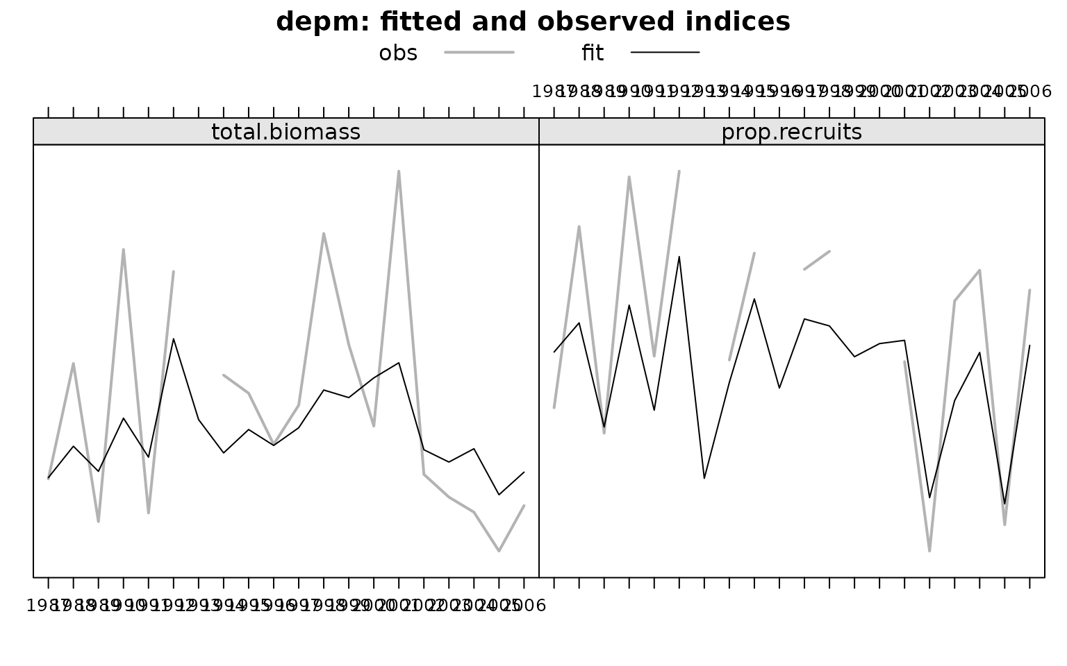
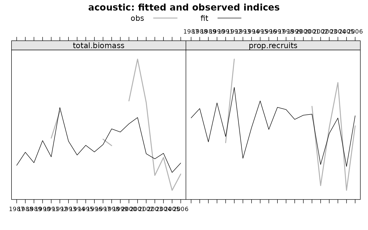
#> units: NAThe fitted object can be plotted:
plot(run) 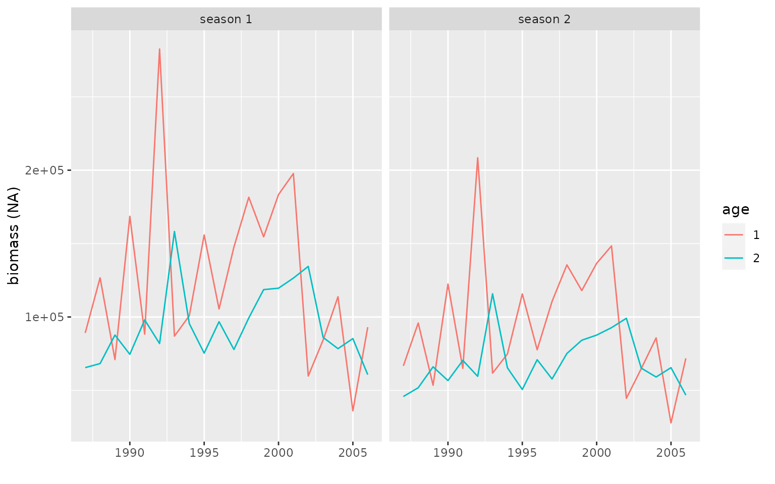
The Pearson residuals can be obtained by:
  res <- residuals(run)
  res
#> An object of class "bbmFitresiduals"
#> Slot "residuals.B":
#> $ depm
#> An object of class "FLQuant"
#> , , unit = unique, season = all, area = unique
#>
#>      year
#> age   1987      1988      1989      1990      1991      1992      1993
#>   all -0.024443  0.961664 -1.256340  1.422196 -1.221749  0.488972        NA
#>      year
#> age   1994      1995      1996      1997      1998      1999      2000
#>   all  0.954562  0.431722  0.014532  0.276855  1.195880  0.507847 -0.544346
#>      year
#> age   2001      2002      2003      2004      2005      2006
#>   all  1.256868 -0.420426 -0.710554 -1.332340 -2.222994 -0.750744
#>
#> units:
#>
#> $ acoustic
#> An object of class "FLQuant"
#> , , unit = unique, season = all, area = unique
#>
#>      year
#> age   1987      1988      1989      1990      1991      1992      1993
#>   all        NA        NA        NA        NA  0.847180 -0.098028        NA
#>      year
#> age   1994      1995      1996      1997      1998      1999      2000
#>   all -0.861658        NA        NA  0.222276 -0.645974        NA  0.651180
#>      year
#> age   2001      2002      2003      2004      2005      2006
#>   all  1.344320  1.802746 -1.122943 -0.216843 -1.936032 -0.770412
#>
#> units:
#>
#>
#> Slot "residuals.P":
#> $ depm
#> An object of class "FLQuant"
#> , , unit = unique, season = all, area = unique
#>
#>      year
#> age   1987      1988      1989      1990      1991      1992      1993
#>   all -0.708038  1.261453 -0.077097  1.723519  0.676241  1.283191        NA
#>      year
#> age   1994      1995      1996      1997      1998      1999      2000
#>   all  0.282155  0.621243        NA  0.653015  0.973985        NA        NA
#>      year
#> age   2001      2002      2003      2004      2005      2006
#>   all -0.274542 -0.721127  1.245323  1.045261 -0.285887  0.706503
#>
#> units:  NA
#>
#> $ acoustic
#> An object of class "FLQuant"
#> , , unit = unique, season = all, area = unique
#>
#>      year
#> age   1987     1988     1989     1990     1991     1992     1993     1994
#>   all       NA       NA       NA       NA -0.25682  1.41182       NA       NA
#>      year
#> age   1995     1996     1997     1998     1999     2000     2001     2002
#>   all       NA       NA -0.33079       NA       NA       NA  0.33385 -0.94820
#>      year
#> age   2003     2004     2005     2006
#>   all  0.24709  1.50004 -1.08214 -0.43049
#>
#> units:  NA
The output object is of class bbmFitresiduals.
  class(res)
#> [1] "bbmFitresiduals"
#> attr(,"package")
#> [1] "bbm"
The class bbmFitresiduals has one slot for the residuals of the indices in biomass (residuals.B) and another one for the percentage of recruits (residuals.P). Both slots are of class FLQuants, with one element per survey index.
  slotNames(res)
#> [1] "residuals.B" "residuals.P"
  res@residuals.B$depm
#> An object of class "FLQuant"
#> , , unit = unique, season = all, area = unique
#>
#>      year
#> age   1987      1988      1989      1990      1991      1992      1993
#>   all -0.024443  0.961664 -1.256340  1.422196 -1.221749  0.488972        NA
#>      year
#> age   1994      1995      1996      1997      1998      1999      2000
#>   all  0.954562  0.431722  0.014532  0.276855  1.195880  0.507847 -0.544346
#>      year
#> age   2001      2002      2003      2004      2005      2006
#>   all  1.256868 -0.420426 -0.710554 -1.332340 -2.222994 -0.750744
#>
#> units:
Then, we can plot the residuals to check that there are no patterns:
plot(res) 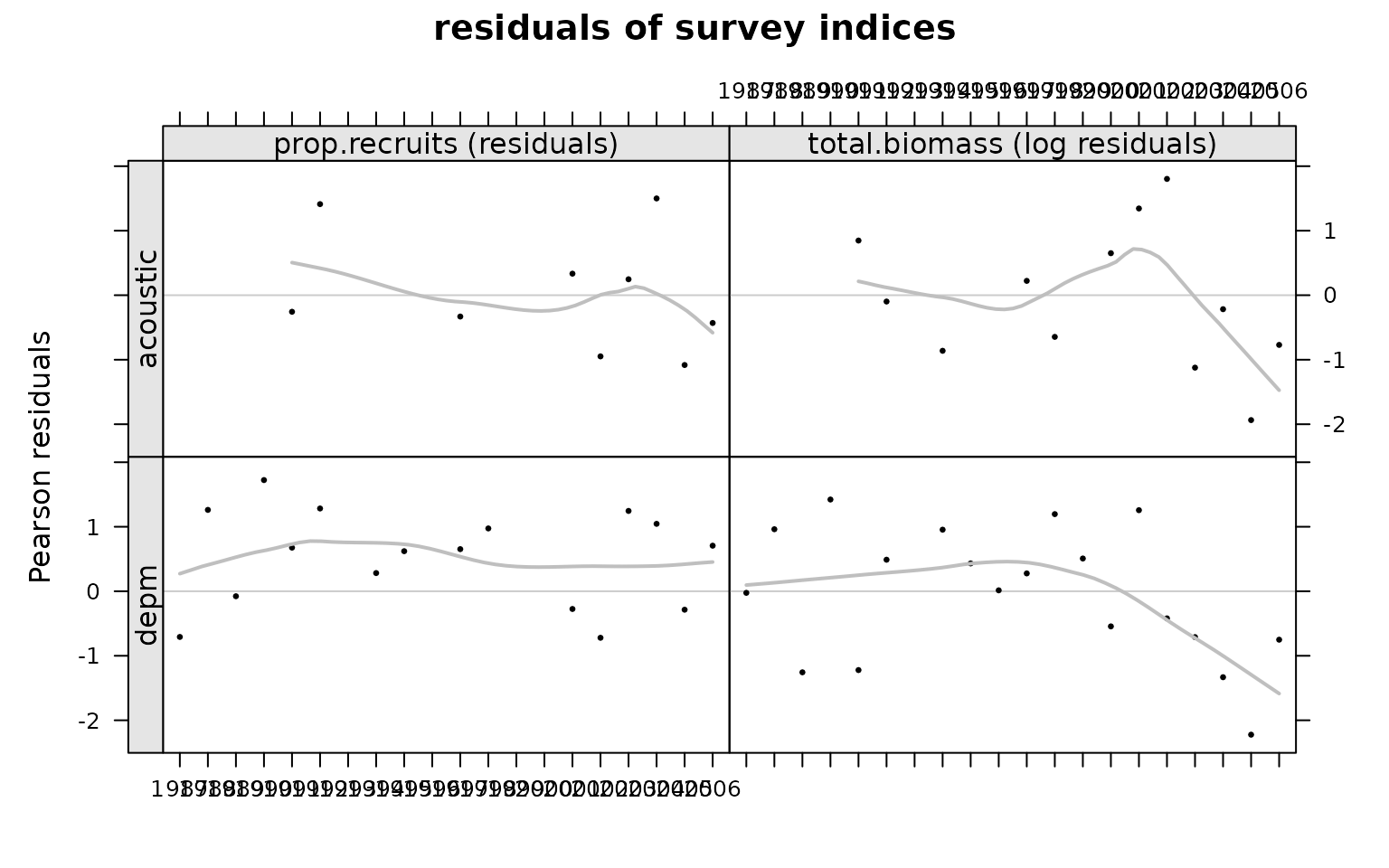
#qqmath(res)Starting from different initial values
The initial values for the optimization could be set by hand or calculated automatically using the function createInits in the package as we will show later. If the optimization works properly the results should be independent of the initial values of the optimization.
In order to create our own initial values, we first generate an empty object with the correct parameter names by using the function bbmFLPar and we then fill it directly with the selected values:
inits.ane2 <- bbmFLPar( years=dimnames(catch.ane)$year, namesB=names(indicesB.ane), namesP=names(indicesP.ane),
                        niter=dim(catch.ane)[6])

inits.ane2[] <- c( 0.6, 0.6, 100, 100, 3, 3, 60000, rep(40000, nyrs), 10, 2)
inits.ane2
#> An object of class "FLPar"
#> params
#>       q_depm   q_acoustic     psi_depm psi_acoustic      xi_depm  xi_acoustic
#>        6e-01        6e-01        1e+02        1e+02        3e+00        3e+00
#>           B0       R_1987       R_1988       R_1989       R_1990       R_1991
#>        6e+04        4e+04        4e+04        4e+04        4e+04        4e+04
#>       R_1992       R_1993       R_1994       R_1995       R_1996       R_1997
#>        4e+04        4e+04        4e+04        4e+04        4e+04        4e+04
#>       R_1998       R_1999       R_2000       R_2001       R_2002       R_2003
#>        4e+04        4e+04        4e+04        4e+04        4e+04        4e+04
#>       R_2004       R_2005       R_2006          mur         psir
#>        4e+04        4e+04        4e+04        1e+01        2e+00
#> units:  NA
Alternatively, initial values can be generated automatically from the dat using the function createInits:
inits.ane3 <- createInits( catch.ane, indicesB=indicesB.ane, indicesP=indicesP.ane,
                           g=control.ane@g)
inits.ane3
#> An object of class "FLPar"
#> params
#>       q_depm   q_acoustic     psi_depm psi_acoustic      xi_depm  xi_acoustic
#>     5.95e-01     8.29e-01     8.78e+00     6.53e+00     2.40e+00     2.32e+00
#>           B0       R_1987       R_1988       R_1989       R_1990       R_1991
#>     3.50e+04     2.90e+04     9.65e+04     1.53e+04     1.72e+05     4.05e+04
#>       R_1992       R_1993       R_1994       R_1995       R_1996       R_1997
#>     1.66e+05     5.78e+04     6.62e+04     8.35e+04     5.78e+04     7.37e+04
#>       R_1998       R_1999       R_2000       R_2001       R_2002       R_2003
#>     1.49e+05     5.78e+04     5.78e+04     1.48e+05     2.40e+04     2.91e+04
#>       R_2004       R_2005       R_2006          mur         psir
#>     4.93e+04     4.05e+03     2.83e+04     1.06e+01     1.29e+00
#> units:  NA
Then, we fit the model starting from different initial values:
  run1 <- bbm(catch.ane, indicesB=indicesB.ane, indicesP=indicesP.ane, control=control.ane, inits=inits.ane)
  run2 <- bbm(catch.ane, indicesB=indicesB.ane, indicesP=indicesP.ane, control=control.ane, inits=inits.ane2)
  run3 <- bbm(catch.ane, indicesB=indicesB.ane, indicesP=indicesP.ane, control=control.ane, inits=inits.ane3)
We can compare the fitted parameters:
  params(run1)
#> An object of class "FLPar"
#> params
#>       q_depm   q_acoustic     psi_depm psi_acoustic      xi_depm  xi_acoustic
#>     2.64e-01     3.44e-01     3.90e+00     7.17e+00     2.24e+00     2.38e+00
#>           B0       R_1987       R_1988       R_1989       R_1990       R_1991
#>     6.55e+04     8.91e+04     1.27e+05     7.10e+04     1.69e+05     8.83e+04
#>       R_1992       R_1993       R_1994       R_1995       R_1996       R_1997
#>     2.83e+05     8.70e+04     1.01e+05     1.56e+05     1.05e+05     1.48e+05
#>       R_1998       R_1999       R_2000       R_2001       R_2002       R_2003
#>     1.82e+05     1.55e+05     1.83e+05     1.98e+05     5.98e+04     8.43e+04
#>       R_2004       R_2005       R_2006          mur         psir
#>     1.14e+05     3.61e+04     9.31e+04     1.16e+01     5.09e+00
#> units:  NA
  params(run2)
#> An object of class "FLPar"
#> params
#>       q_depm   q_acoustic     psi_depm psi_acoustic      xi_depm  xi_acoustic
#>     8.26e-01     1.10e+00     8.84e+00     7.11e+00     5.37e+00     2.63e+00
#>           B0       R_1987       R_1988       R_1989       R_1990       R_1991
#>     2.24e+04     1.76e+04     4.58e+04     1.42e+04     9.27e+04     2.85e+04
#>       R_1992       R_1993       R_1994       R_1995       R_1996       R_1997
#>     1.41e+05     8.90e+04     5.02e+04     5.64e+04     6.88e+04     5.85e+04
#>       R_1998       R_1999       R_2000       R_2001       R_2002       R_2003
#>     8.99e+04     7.34e+04     1.40e+05     8.27e+04     1.45e+04     3.12e+04
#>       R_2004       R_2005       R_2006          mur         psir
#>     4.56e+04     6.82e+03     2.93e+04     1.08e+01     2.14e+00
#> units:  NA
  params(run3)
#> An object of class "FLPar"
#> params
#>       q_depm   q_acoustic     psi_depm psi_acoustic      xi_depm  xi_acoustic
#>     9.08e-01     1.76e+00     1.45e+01     1.43e+00     8.16e+00     3.35e+00
#>           B0       R_1987       R_1988       R_1989       R_1990       R_1991
#>     2.10e+04     1.68e+04     4.04e+04     1.08e+04     8.48e+04     2.43e+04
#>       R_1992       R_1993       R_1994       R_1995       R_1996       R_1997
#>     1.04e+05     1.14e+05     5.05e+04     5.91e+04     6.51e+04     5.40e+04
#>       R_1998       R_1999       R_2000       R_2001       R_2002       R_2003
#>     8.01e+04     9.10e+04     1.28e+05     7.79e+04     1.09e+04     2.60e+04
#>       R_2004       R_2005       R_2006          mur         psir
#>     3.29e+04     3.52e+03     1.54e+04     1.08e+01     1.49e+00
#> units:  NA
And the corresponding AIC values:
The time series of estimated recruits can be plotted:
parnames <- sapply(dimnames(run1@params)$params, function(x) unlist(strsplit(x,split="_"))[1])
dat <- cbind( run1=c(params(run1)[parnames %in% "R"]), run2=c(params(run2)[parnames %in% "R"]),
              run3=c(params(run3)[parnames %in% "R"]))
rownames(dat) <- years

matplot( dat, type="l", ylab="R (t)", xlab="year", lty=1, col=c('black','red','green'), xaxt = "n")
axis(1, at=1:nyrs, labels=years)
legend( "topright", paste("run",1:3,sep=""), lty=1:3, col=c('black','red','green'), bty="n")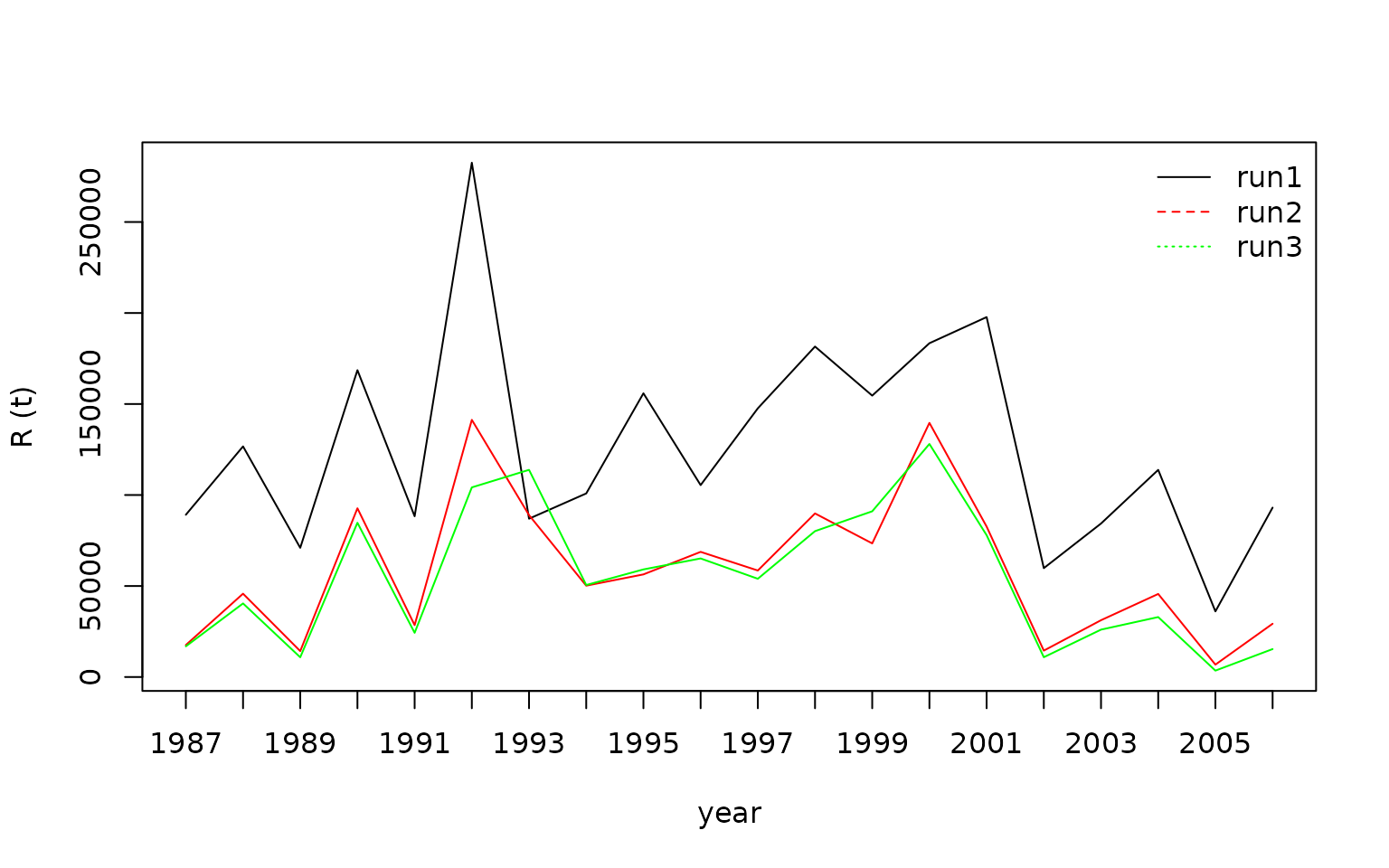
Fixing some parameters
Any of the model parameterscan be fixed by setting its param.fix value equal to 1. Then, the parameter will be fixed to the initial value and won’t be estimated.
We fix the catchability of the biomass estimate from the depm survey, as follows:
param.fix <- bbmFLPar( 0, years=dimnames(catch.ane)$year, niter=dim(catch.ane)[6],
                       namesB=names(indicesB.ane), namesP=names(indicesP.ane))
param.fix['q_depm'] <- 1

control.ane2 <- bbmControl(g=c(rec=0.68, adult=0.68), param.fix=param.fix)
  run4 <- bbm( catch.ane, indicesB=indicesB.ane, indicesP=indicesP.ane,
               control=control.ane2, inits=inits.ane)
The estimated parameters and their corresponding standard errors are:
  params(run4)
#> An object of class "FLPar"
#> params
#>       q_depm   q_acoustic     psi_depm psi_acoustic      xi_depm  xi_acoustic
#>     1.00e+00     5.02e-01     1.40e+00     3.96e+00     1.95e+00     1.06e+00
#>           B0       R_1987       R_1988       R_1989       R_1990       R_1991
#>     2.99e+04     6.92e+04     7.48e+04     6.85e+04     9.40e+04     6.50e+04
#>       R_1992       R_1993       R_1994       R_1995       R_1996       R_1997
#>     1.10e+05     8.82e+04     7.87e+04     7.91e+04     8.40e+04     7.94e+04
#>       R_1998       R_1999       R_2000       R_2001       R_2002       R_2003
#>     8.54e+04     8.87e+04     1.02e+05     9.41e+04     5.78e+04     6.68e+04
#>       R_2004       R_2005       R_2006          mur         psir
#>     8.85e+04     5.56e+04     7.48e+04     1.13e+01     2.12e+01
#> units:  NA
  params.se(run4)
#> An object of class "FLPar"
#> params
#>       q_depm   q_acoustic     psi_depm psi_acoustic      xi_depm  xi_acoustic
#>     0.00e+00     1.23e-01     5.11e-01     1.57e+00     2.75e-01     4.95e-01
#>           B0       R_1987       R_1988       R_1989       R_1990       R_1991
#>     1.66e+04     1.45e+04     1.69e+04     1.41e+04     2.09e+04     1.30e+04
#>       R_1992       R_1993       R_1994       R_1995       R_1996       R_1997
#>     2.57e+04     1.92e+04     1.66e+04     1.91e+04     1.87e+04     1.83e+04
#>       R_1998       R_1999       R_2000       R_2001       R_2002       R_2003
#>     2.09e+04     2.28e+04     2.27e+04     1.95e+04     8.83e+03     1.42e+04
#>       R_2004       R_2005       R_2006          mur         psir
#>     2.28e+04     8.69e+03     1.80e+04     1.40e-01          NaN
#> units:  NA
Where, values for the q_depm parameter are:
  inits.ane$q_depm
#> An object of class "FLPar"
#> params
#> q_depm
#>      1
#> units:  NA
  run4@params$q_depm
#> An object of class "FLPar"
#> params
#> q_depm
#>      1
#> units:  NA
  run4@params.se$q_depm
#> An object of class "FLPar"
#> params
#> q_depm
#>      0
#> units:  NA
Simulated data set
The package also includes a function to simulate data. Say, that we want to create biomass and recruits proportion indices from a survey conducted at mid-year. So the year is separated into two seasons. First, we need an FLQuant with the catch in biomass for the recruits and the adults in each of the seasons. Starting from the landings of ple4, we can generate it as follows:
data(ple4)

aux <- landings.n(ple4)*landings.wt(ple4)
catch.ple4 <- FLQuant(NA, dim=c(2, dim(landings.n(ple4))[2], 1, 2, 1, 1), dimnames=list(year=dimnames(landings.n(ple4))$year))
catch.ple4[1, , ,1:2, ,] <- aux[1,]/2
catch.ple4[2, , ,1:2, , ] <- quantSums(aux[-1,])/2
catch.ple4
#> An object of class "FLQuant"
#> , , unit = unique, season = 1, area = unique
#>
#>      year
#> quant 1957       1958       1959       1960       1961       1962
#>     1 0.0000e+00 0.0000e+00 0.0000e+00 0.0000e+00 0.0000e+00 0.0000e+00
#>     2 3.5463e+04 3.7078e+04 3.9089e+04 4.4382e+04 4.2633e+04 4.5152e+04
#>      year
#> quant 1963       1964       1965       1966       1967       1968
#>     1 0.0000e+00 0.0000e+00 0.0000e+00 0.0000e+00 0.0000e+00 0.0000e+00
#>     2 5.1581e+04 5.5560e+04 5.2712e+04 4.9167e+04 5.1974e+04 6.0510e+04
#>      year
#> quant 1969       1970       1971       1972       1973       1974
#>     1 5.1204e-01 1.1202e+01 2.7188e+00 2.3863e+02 3.3353e+02 3.3284e+02
#>     2 6.1330e+04 5.5880e+04 5.8648e+04 6.4983e+04 6.6551e+04 5.7258e+04
#>      year
#> quant 1975       1976       1977       1978       1979       1980
#>     1 9.9018e+01 3.8363e+02 4.9032e+02 1.5356e+02 1.2469e+02 1.1899e+02
#>     2 4.7130e+04 6.0699e+04 5.3772e+04 6.4029e+04 5.9789e+04 7.5201e+04
#>      year
#> quant 1981       1982       1983       1984       1985       1986
#>     1 4.2440e+01 4.2995e+02 1.4442e+02 1.3322e+01 1.7098e+01 1.7853e+02
#>     2 7.5610e+04 7.2405e+04 7.1701e+04 8.1327e+04 9.1170e+04 8.3138e+04
#>      year
#> quant 1987       1988       1989       1990       1991       1992
#>     1 0.0000e+00 0.0000e+00 1.6920e+02 2.9302e+02 1.6473e+02 5.0245e+02
#>     2 7.7503e+04 8.4059e+04 9.3664e+04 8.6914e+04 7.3757e+04 6.6894e+04
#>      year
#> quant 1993       1994       1995       1996       1997       1998
#>     1 4.4603e+02 2.3132e+02 1.0598e+03 1.2398e+02 1.9618e+02 1.3022e+01
#>     2 7.0454e+04 6.2866e+04 5.3781e+04 4.6697e+04 4.1241e+04 3.7096e+04
#>      year
#> quant 1999       2000       2001       2002       2003       2004
#>     1 4.8084e+01 3.5965e+02 1.5050e+03 1.2782e+02 1.0888e+02 5.8620e+01
#>     2 4.8622e+04 4.9799e+04 3.1793e+04 4.3441e+04 3.7276e+04 4.1206e+04
#>      year
#> quant 2005       2006       2007       2008       2009       2010
#>     1 7.1384e+02 3.0810e+01 4.5589e+02 5.7065e+01 1.5311e+02 2.6748e+02
#>     2 3.0037e+04 3.1050e+04 2.9401e+04 3.2230e+04 3.4268e+04 3.6856e+04
#>      year
#> quant 2011       2012       2013       2014       2015       2016
#>     1 6.6115e+01 2.0601e+01 8.5741e+00 5.5005e-01 0.0000e+00 0.0000e+00
#>     2 3.7152e+04 4.1133e+04 4.8553e+04 4.3211e+04 4.5517e+04 4.3191e+04
#>      year
#> quant 2017
#>     1 2.5690e+00
#>     2 4.2372e+04
#>
#> , , unit = unique, season = 2, area = unique
#>
#>      year
#> quant 1957       1958       1959       1960       1961       1962
#>     1 0.0000e+00 0.0000e+00 0.0000e+00 0.0000e+00 0.0000e+00 0.0000e+00
#>     2 3.5463e+04 3.7078e+04 3.9089e+04 4.4382e+04 4.2633e+04 4.5152e+04
#>      year
#> quant 1963       1964       1965       1966       1967       1968
#>     1 0.0000e+00 0.0000e+00 0.0000e+00 0.0000e+00 0.0000e+00 0.0000e+00
#>     2 5.1581e+04 5.5560e+04 5.2712e+04 4.9167e+04 5.1974e+04 6.0510e+04
#>      year
#> quant 1969       1970       1971       1972       1973       1974
#>     1 5.1204e-01 1.1202e+01 2.7188e+00 2.3863e+02 3.3353e+02 3.3284e+02
#>     2 6.1330e+04 5.5880e+04 5.8648e+04 6.4983e+04 6.6551e+04 5.7258e+04
#>      year
#> quant 1975       1976       1977       1978       1979       1980
#>     1 9.9018e+01 3.8363e+02 4.9032e+02 1.5356e+02 1.2469e+02 1.1899e+02
#>     2 4.7130e+04 6.0699e+04 5.3772e+04 6.4029e+04 5.9789e+04 7.5201e+04
#>      year
#> quant 1981       1982       1983       1984       1985       1986
#>     1 4.2440e+01 4.2995e+02 1.4442e+02 1.3322e+01 1.7098e+01 1.7853e+02
#>     2 7.5610e+04 7.2405e+04 7.1701e+04 8.1327e+04 9.1170e+04 8.3138e+04
#>      year
#> quant 1987       1988       1989       1990       1991       1992
#>     1 0.0000e+00 0.0000e+00 1.6920e+02 2.9302e+02 1.6473e+02 5.0245e+02
#>     2 7.7503e+04 8.4059e+04 9.3664e+04 8.6914e+04 7.3757e+04 6.6894e+04
#>      year
#> quant 1993       1994       1995       1996       1997       1998
#>     1 4.4603e+02 2.3132e+02 1.0598e+03 1.2398e+02 1.9618e+02 1.3022e+01
#>     2 7.0454e+04 6.2866e+04 5.3781e+04 4.6697e+04 4.1241e+04 3.7096e+04
#>      year
#> quant 1999       2000       2001       2002       2003       2004
#>     1 4.8084e+01 3.5965e+02 1.5050e+03 1.2782e+02 1.0888e+02 5.8620e+01
#>     2 4.8622e+04 4.9799e+04 3.1793e+04 4.3441e+04 3.7276e+04 4.1206e+04
#>      year
#> quant 2005       2006       2007       2008       2009       2010
#>     1 7.1384e+02 3.0810e+01 4.5589e+02 5.7065e+01 1.5311e+02 2.6748e+02
#>     2 3.0037e+04 3.1050e+04 2.9401e+04 3.2230e+04 3.4268e+04 3.6856e+04
#>      year
#> quant 2011       2012       2013       2014       2015       2016
#>     1 6.6115e+01 2.0601e+01 8.5741e+00 5.5005e-01 0.0000e+00 0.0000e+00
#>     2 3.7152e+04 4.1133e+04 4.8553e+04 4.3211e+04 4.5517e+04 4.3191e+04
#>      year
#> quant 2017
#>     1 2.5690e+00
#>     2 4.2372e+04
#>
#> units:  NA
We assume that the true values of the model parameters we are going to use to simulate are:
rr <- rlnorm(dim(catch.ple4)[2], log(300000), 1/sqrt(3))
par.ple4 <- bbmFLPar(years=dimnames(catch.ple4)$year, namesB=c("Mysurvey"), namesP=c("Mysurvey"), niter=1)
par.ple4[] <- c(1, 200, 4, 200000, rr, log(250000), 3)
par.ple4
#> An object of class "FLPar"
#> params
#>   q_Mysurvey psi_Mysurvey  xi_Mysurvey           B0       R_1957       R_1958
#>          1.0        200.0          4.0     200000.0     290285.7     350606.3
#>       R_1959       R_1960       R_1961       R_1962       R_1963       R_1964
#>     497034.2     268778.0     566383.1     179068.9     172851.3     183030.5
#>       R_1965       R_1966       R_1967       R_1968       R_1969       R_1970
#>     157776.6     142556.1     464628.1     180890.9     828013.4     298327.2
#>       R_1971       R_1972       R_1973       R_1974       R_1975       R_1976
#>     231576.0     280126.1     230627.5     151521.1     230655.3     538988.5
#>       R_1977       R_1978       R_1979       R_1980       R_1981       R_1982
#>     771862.3     181344.7     122420.3     448591.3     312614.1     156965.9
#>       R_1983       R_1984       R_1985       R_1986       R_1987       R_1988
#>     417667.7     236575.6     126871.9     245904.4     291176.3     498512.2
#>       R_1989       R_1990       R_1991       R_1992       R_1993       R_1994
#>     888325.0     889173.7     421680.3     434795.0     246171.5     589753.8
#>       R_1995       R_1996       R_1997       R_1998       R_1999       R_2000
#>     631154.5     181925.7     396787.6     802382.1     144403.8     180565.0
#>       R_2001       R_2002       R_2003       R_2004       R_2005       R_2006
#>     723529.1     343618.8     270193.7     716677.4     254756.7     644973.8
#>       R_2007       R_2008       R_2009       R_2010       R_2011       R_2012
#>     739758.5     272763.4     113021.9     162676.2     330606.6     465717.5
#>       R_2013       R_2014       R_2015       R_2016       R_2017          mur
#>     494461.6     498954.3     564394.8     377035.8     890576.1         12.4
#>         psir
#>          3.0
#> units:  NA
And the true values of the biomass change rates for recruits and adults are:
g <- c(rec=0.3, adult=0.25)We can compute the true values of recruits and adults biomass at the beginning of each season and check that these values are large enough to support the observed levels of catches (i.e. there are no negative biomasses):
pop.ple4 <- calcPop(g=g, f=c(0.5, 0.5), catch=catch.ple4, inits=par.ple4)
pop.ple4
#> $stock.bio
#> An object of class "FLQuant"
#> , , unit = unique, season = 1, area = unique
#>
#>      year
#> quant 1957    1958    1959    1960    1961    1962    1963    1964    1965
#>     1  290286  350606  497034  268778  566383  179069  172851  183031  157777
#>     2  200000  308095  434109  637170  616857  824601  695008  578106  487567
#>      year
#> quant 1966    1967    1968    1969    1970    1971    1972    1973    1974
#>     1  142556  464628  180891  828013  298327  231576  280126  230628  151521
#>     2  403383  332815  511489  425347  836208  773405  670165  614117  530861
#>      year
#> quant 1975    1976    1977    1978    1979    1980    1981    1982    1983
#>     1  230655  538988  771862  181345  122420  448591  312614  156966  417668
#>     2  423853  417453  616400  955924  765321  580776  651439  605147  458787
#>      year
#> quant 1984    1985    1986    1987    1988    1989    1990    1991    1992
#>     1  236576  126872  245904  291176  498512  888325  889174  421680  434795
#>     2  539672  451710  284523  256424  278353  437435  832831 1153117 1079718
#>      year
#> quant 1993    1994    1995    1996    1997    1998    1999    2000    2001
#>     1  246171  589754  631154  181926  396788  802382  144404  180565  723529
#>     2 1043823  869935 1002832 1151640  948877  959662 1276181 1014800  835405
#>      year
#> quant 2002    2003    2004    2005    2006    2007    2008    2009    2010
#>     1  343619  270194  716677  254757  644974  739759  272763  113022  162676
#>     2 1127795 1055843  956347 1202761 1071089 1257010 1474207 1293086 1029920
#>      year
#> quant 2011    2012    2013    2014    2015    2016    2017
#>     1  330607  465718  494462  498954  564395  377036  890576
#>     2  856978  846518  931505 1005885 1076600 1176078 1118865
#>
#> , , unit = unique, season = 2, area = unique
#>
#>      year
#> quant 1957    1958    1959    1960    1961    1962    1963    1964    1965
#>     1  249851  301770  427801  231339  487490  154126  148774  157536  135800
#>     2  143185  237061  346379  520607  504324  685291  564886  457983  380758
#>      year
#> quant 1966    1967    1968    1969    1970    1971    1972    1973    1974
#>     1  122699  399909  155694  712677  256762  199317  240885  198194  130107
#>     2  309796  244883  394543  317753  685456  627434  530373  479438  414695
#>      year
#> quant 1975    1976    1977    1978    1979    1980    1981    1982    1983
#>     1  198435  463556  663893  155942  105252  385996  269030  134703  359356
#>     2  329775  311380  493458  783450  619227  441888  503864  466022  337521
#>      year
#> quant 1984    1985    1986    1987    1988    1989    1990    1991    1992
#>     1  203610  109184  211486  250618  429073  764431  765047  362791  373765
#>     2  399858  312987  172990  153486  166679  298046  653322  948334  890006
#>      year
#> quant 1993    1994    1995    1996    1997    1998    1999    2000    2001
#>     1  211468  507391  542256  156470  341336  690605  124245  155080  621351
#>     2  854985  708658  834474  972451  798638  812050 1080550  848776  707376
#>      year
#> quant 2002    2003    2004    2005    2006    2007    2008    2009    2010
#>     1  295637  232457  616796  218609  555105  636293  234717   97137  139769
#>     2  954467  896760  805264 1033216  916064 1081688 1270706 1108953  874279
#>      year
#> quant 2011    2012    2013    2014    2015    2016    2017
#>     1  284494  400828  425579  429453  485779  324518  766524
#>     2  721379  708409  776439  847097  907338  997311  947590
#>
#> units:  NA
#>
#> $ok
#> [1] TRUE
The observed indices of total biomass and recruits biomass proportion of a survey named “Mysurvey” conduceted at the middle of the year are generated as follows:
indices.ple4 <- simIndices( catch.ple4, g=g, inits=par.ple4,
                         findicesB=c(Mysurvey=0.5), findicesP=c(Mysurvey=0.5) )
The resulting object is a list of two FLIndices: one for the total biomass indices and one for the recruits biomass proportions:
length(indices.ple4)
#> [1] 2
names(indices.ple4)
#> [1] "Btot" "Prec"

lapply(indices.ple4$Btot, index)
#> $ Mysurvey
#> An object of class "FLQuant"
#> , , unit = unique, season = all, area = unique
#>
#>      year
#> age   1957    1958    1959    1960    1961    1962    1963    1964    1965
#>   all  414297  533734  687043  691667  980188  862673  699962  643095  479560
#>      year
#> age   1966    1967    1968    1969    1970    1971    1972    1973    1974
#>   all  399495  580287  578080 1109162  859598  859055  698836  704344  539595
#>      year
#> age   1975    1976    1977    1978    1979    1980    1981    1982    1983
#>   all  532908  761876 1239954  946744  714657  797254  852350  561175  677740
#>      year
#> age   1984    1985    1986    1987    1988    1989    1990    1991    1992
#>   all  525497  479257  393948  410850  584449 1067577 1315794 1333217 1162205
#>      year
#> age   1993    1994    1995    1996    1997    1998    1999    2000    2001
#>   all 1011371 1198110 1339235 1284557 1190238 1394418 1287995 1071732 1212102
#>      year
#> age   2002    2003    2004    2005    2006    2007    2008    2009    2010
#>   all 1229408 1294121 1425464 1355778 1526242 1456490 1411345 1216395 1086381
#>      year
#> age   2011    2012    2013    2014    2015    2016    2017
#>   all  949426 1064512 1158446 1336268 1404537 1530766 1767450
#>
#> units:  NA
lapply(indices.ple4$Btot, range)
#> $Mysurvey
#>       min       max plusgroup   minyear   maxyear    startf      endf
#>        NA        NA        NA    1957.0    2017.0       0.5       0.5
lapply(indices.ple4$Prec, index)
#> $ Mysurvey
#> An object of class "FLQuant"
#> , , unit = unique, season = all, area = unique
#>
#>      year
#> age   1957     1958     1959     1960     1961     1962     1963     1964
#>   all 0.635608 0.560085 0.552471 0.307722 0.491509 0.183657 0.208386 0.255946
#>      year
#> age   1965     1966     1967     1968     1969     1970     1971     1972
#>   all 0.262990 0.283827 0.620206 0.282936 0.691576 0.272465 0.241067 0.312332
#>      year
#> age   1973     1974     1975     1976     1977     1978     1979     1980
#>   all 0.292598 0.238973 0.375729 0.598123 0.573588 0.165979 0.145268 0.466423
#>      year
#> age   1981     1982     1983     1984     1985     1986     1987     1988
#>   all 0.348220 0.224223 0.515658 0.337422 0.258742 0.549983 0.620118 0.720278
#>      year
#> age   1989     1990     1991     1992     1993     1994     1995     1996
#>   all 0.719452 0.539472 0.276715 0.295726 0.198193 0.417262 0.393941 0.138544
#>      year
#> age   1997     1998     1999     2000     2001     2002     2003     2004
#>   all 0.299399 0.459570 0.103048 0.154550 0.467739 0.236504 0.205846 0.433769
#>      year
#> age   2005     2006     2007     2008     2009     2010     2011     2012
#>   all 0.174588 0.377322 0.370386 0.155929 0.080574 0.137853 0.282776 0.361386
#>      year
#> age   2013     2014     2015     2016     2017
#>   all 0.354040 0.336421 0.348697 0.245433 0.447247
#>
#> units:  NA
lapply(indices.ple4$Prec, range)
#> $Mysurvey
#>       min       max plusgroup   minyear   maxyear    startf      endf
#>        NA        NA        NA    1957.0    2017.0       0.5       0.5
Now, we can prepare the elements necessary to fit the model to these indices. Basically, we need a bbmControl object and an FLPar with initial parameters:
param.fix <- par.ple4
param.fix[] <- 0 # dummy FLPar indicating which parameters are fixed (0 estimated and 1 fixed)

control.ple4 <- new( "bbmControl", g=g, param.fix=param.fix)  # bbmControl. We assumed g is known exactly

inits.ple4 <- createInits(catch.ple4, indicesB=indices.ple4$Btot, indicesP=indices.ple4$Prec, g=g) # create automatic initial parameters
Then, the model is fitted as follows:
fit.ple4 <- bbm(catch.ple4, indicesB=indices.ple4$Btot, indicesP=indices.ple4$Prec,
                control=control.ple4, inits=inits.ple4)
We can check the results
params(fit.ple4)
#> An object of class "FLPar"
#> params
#>   q_Mysurvey psi_Mysurvey  xi_Mysurvey           B0       R_1957       R_1958
#>     9.97e-01     2.35e+02     7.89e+00     2.11e+05     3.00e+05     3.46e+05
#>       R_1959       R_1960       R_1961       R_1962       R_1963       R_1964
#>     4.64e+05     2.51e+05     5.37e+05     1.83e+05     1.71e+05     1.89e+05
#>       R_1965       R_1966       R_1967       R_1968       R_1969       R_1970
#>     1.52e+05     1.37e+05     4.26e+05     1.84e+05     8.45e+05     2.81e+05
#>       R_1971       R_1972       R_1973       R_1974       R_1975       R_1976
#>     2.39e+05     2.64e+05     2.32e+05     1.53e+05     2.28e+05     5.19e+05
#>       R_1977       R_1978       R_1979       R_1980       R_1981       R_1982
#>     7.85e+05     1.88e+05     1.23e+05     4.29e+05     3.27e+05     1.53e+05
#>       R_1983       R_1984       R_1985       R_1986       R_1987       R_1988
#>     4.18e+05     2.20e+05     1.34e+05     2.58e+05     3.04e+05     5.11e+05
#>       R_1989       R_1990       R_1991       R_1992       R_1993       R_1994
#>     8.58e+05     8.39e+05     4.25e+05     4.11e+05     2.39e+05     5.71e+05
#>       R_1995       R_1996       R_1997       R_1998       R_1999       R_2000
#>     5.97e+05     1.91e+05     3.99e+05     7.60e+05     1.48e+05     1.88e+05
#>       R_2001       R_2002       R_2003       R_2004       R_2005       R_2006
#>     6.84e+05     3.29e+05     2.91e+05     7.02e+05     2.69e+05     6.57e+05
#>       R_2007       R_2008       R_2009       R_2010       R_2011       R_2012
#>     6.84e+05     2.67e+05     1.14e+05     1.74e+05     3.25e+05     4.67e+05
#>       R_2013       R_2014       R_2015       R_2016       R_2017          mur
#>     4.87e+05     5.17e+05     5.79e+05     4.22e+05     9.54e+05     1.28e+01
#>         psir
#>     3.00e+00
#> units:  NA
params.se(fit.ple4)
#> An object of class "FLPar"
#> params
#>   q_Mysurvey psi_Mysurvey  xi_Mysurvey           B0       R_1957       R_1958
#>     1.35e-02     4.89e+01          NaN     5.73e+03     8.28e+03     1.01e+04
#>       R_1959       R_1960       R_1961       R_1962       R_1963       R_1964
#>     1.21e+04     9.01e+03     1.36e+04     7.77e+03     7.00e+03     6.69e+03
#>       R_1965       R_1966       R_1967       R_1968       R_1969       R_1970
#>     5.71e+03     5.21e+03     9.94e+03     7.00e+03     1.80e+04     1.01e+04
#>       R_1971       R_1972       R_1973       R_1974       R_1975       R_1976
#>     8.88e+03     8.77e+03     8.04e+03     6.07e+03     7.80e+03     1.40e+04
#>       R_1977       R_1978       R_1979       R_1980       R_1981       R_1982
#>     1.79e+04     8.44e+03     6.20e+03     1.11e+04     9.48e+03     6.19e+03
#>       R_1983       R_1984       R_1985       R_1986       R_1987       R_1988
#>     9.62e+03     6.45e+03     4.47e+03     5.86e+03     7.52e+03     1.34e+04
#>       R_1989       R_1990       R_1991       R_1992       R_1993       R_1994
#>     2.15e+04     2.21e+04     1.57e+04     1.51e+04     1.09e+04     1.89e+04
#>       R_1995       R_1996       R_1997       R_1998       R_1999       R_2000
#>     1.99e+04     9.74e+03     1.53e+04     2.30e+04     8.82e+03     9.32e+03
#>       R_2001       R_2002       R_2003       R_2004       R_2005       R_2006
#>     2.13e+04     1.42e+04     1.24e+04     2.32e+04     1.25e+04     2.26e+04
#>       R_2007       R_2008       R_2009       R_2010       R_2011       R_2012
#>     2.21e+04     1.35e+04     7.79e+03     8.92e+03     1.33e+04     1.77e+04
#>       R_2013       R_2014       R_2015       R_2016       R_2017          mur
#>     1.92e+04     2.16e+04     2.54e+04     2.05e+04     4.64e+04     7.67e-02
#>         psir
#>     5.62e-01
#> units:  NA
logLik(fit.ple4)
#> 'log Lik.' 210.5291 (df=67)
AIC(fit.ple4)
#> [1] -287.0582
BIC(fit.ple4)
#> [1] -145.6297
(params(fit.ple4) - par.ple4)/par.ple4
#> An object of class "FLPar"
#> params
#>   q_Mysurvey psi_Mysurvey  xi_Mysurvey           B0       R_1957       R_1958
#>     -0.00267      0.17737      0.97132      0.05455      0.03350     -0.01434
#>       R_1959       R_1960       R_1961       R_1962       R_1963       R_1964
#>     -0.06657     -0.06611     -0.05242      0.01920     -0.00845      0.03039
#>       R_1965       R_1966       R_1967       R_1968       R_1969       R_1970
#>     -0.03957     -0.03706     -0.08238      0.01603      0.02109     -0.05969
#>       R_1971       R_1972       R_1973       R_1974       R_1975       R_1976
#>      0.03229     -0.05876      0.00772      0.01149     -0.00948     -0.03659
#>       R_1977       R_1978       R_1979       R_1980       R_1981       R_1982
#>      0.01719      0.03465      0.00729     -0.04310      0.04713     -0.02609
#>       R_1983       R_1984       R_1985       R_1986       R_1987       R_1988
#>      0.00131     -0.06803      0.05677      0.04741      0.04316      0.02491
#>       R_1989       R_1990       R_1991       R_1992       R_1993       R_1994
#>     -0.03435     -0.05661      0.00864     -0.05531     -0.02846     -0.03199
#>       R_1995       R_1996       R_1997       R_1998       R_1999       R_2000
#>     -0.05351      0.05229      0.00479     -0.05267      0.02505      0.04295
#>       R_2001       R_2002       R_2003       R_2004       R_2005       R_2006
#>     -0.05466     -0.04177      0.07703     -0.02022      0.05747      0.01915
#>       R_2007       R_2008       R_2009       R_2010       R_2011       R_2012
#>     -0.07480     -0.02010      0.01047      0.06918     -0.01563      0.00341
#>       R_2013       R_2014       R_2015       R_2016       R_2017          mur
#>     -0.01432      0.03634      0.02651      0.11969      0.07155      0.02990
#>         psir
#>      0.00015
#> units:  NA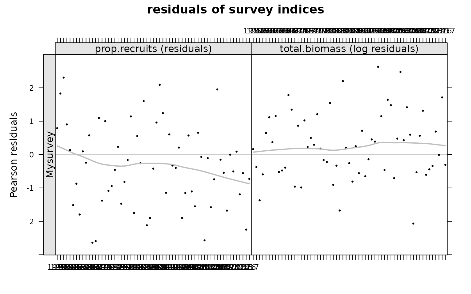
qqmath(res)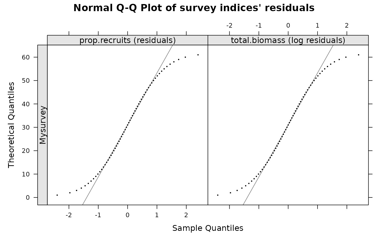
More information
- You can submit bug reports, questions or suggestions on
bbmat thebbmissue page,1 or on the FLR mailing list. - Or send a pull request to https://github.com/flr/bbm/
- For more information on the FLR Project for Quantitative Fisheries Science in R, visit the FLR webpage.2
- The latest version of
bbmcan always be installed using thedevtoolspackage, by calling
References
Giannoulaki, M., L. Ibaibarriaga, K. Antonakakis, A. Uriarte, A. Machias, S. Somarakis, S. Sanchez, and B. Roel. 2014. “Applying a Two-Stage Bayesian Dynamic Model to a Short-Lived Species, the Anchovy, in the Aegean Sea (Eastern Mediterranean). Comparison with an Integrated Catch at Age Stock Assessment Model.” Mediterranean Marine Science 15: 350–65.
Gras, M., B. A. Roel, F. Coppin, E. Foucher, and J. P. Robin. 2014. “A Two-Stage Biomass Model to Assess the English Channel Cuttlefish (Sepia Officinalis L.) Stock.” ICES J. Of Mar. Sci. 64: 640–46.
Ibaibarriaga, L., C. Fernandez, A. Uriarte, and B. Roel. 2008. “A Two-Stage Biomass Dynamic Model for Bay of Biscay Anchovy: A Bayesian Approach.” ICES J. Of Mar. Sci. 65: 191–205.
Kell, L. T., I. Mosqueira, P. Grosjean, J-M. Fromentin, D. Garcia, R. Hillary, E. Jardim, et al. 2007. “FLR: An Open-Source Framework for the Evaluation and Development of Management Strategies.” ICES J. Of Mar. Sci. 64: 640–46.
Kristensen, K., A. Nielsen, C. W. Berg, H. Skaug, and B. M. Bell. 2016. “TMB: Automatic Differentiation and Laplace Approximation.” Journal of Statistical Software 70 (5): 1–21.
Roel, B. A., and D. S. Butterworth. 2000. “Assessment of the South African Chokka Squid Loligo Vulgaris Reynaudii. Is Disturbance of Aggregations by the Recent Jig Fishery Having a Negative Impact on Recruitment?” Fisheries Research 48: 213–28.
Roel, B. A., J. A. A. De Oliveira, and S. Beggs. 2009. “A Two-Stage Biomass Model for Irish Sea Herring Allowing for Additional Variance in the Recruitment Caused by Mixing of Stocks.” ICES J. Of Mar. Sci. 66: 1808–13.