FLife
Modelling Life History relationships
Laurence Kell
30 August, 2022
FLife-full.RmdIntroduction
Life History Relationships
Dynamics
Simulation
More Information
References
Introduction
Life history traits include growth rate; age and size at sexual maturity; the temporal pattern or schedule of reproduction; the number, size, and sex ratio of offspring; the distribution of intrinsic or extrinsic mortality rates (e.g., patterns of senescence); and patterns of dormancy and dispersal. These traits contribute directly to age-specific survival and reproductive functions.1 The FLife package has a variety of methods for modelling life history traits and functional forms for processes for use in fish stock assessment and for conducting Management Strategy Evaluation (MSE).
These relationships have many uses, for example in age-structured population models, functional relationships for these processes allow the calculation of the population growth rate and have been used to to develop priors in stock assesments and to parameterise ecological models.
The FLife package has methods for modelling functional forms, for simulating equilibrium FLBRP and dynamic stock objects FLStock.
Quick Start
This section provide a quick way to get running and provides an overview of the functions available, their potential use, and where to seek help.
A number of packages need to be installed from CRAN and the
FLR website, where tutorials are also available.
Extensive use is made of the packages of Hadley Wickham. For example ggplot2, based on the Grammar of Graphics,2 is used for plotting3. While reshape and plyr are used for data manipulatation and analysis.
The simplest way to obtain FLife is to install it from the FLR repository via the R console. See help(install.packages) for more details.
install.packages("FLife", repos = "http://flr-project.org/R")After installing the FLife package load it
library(FLife)Life History Relationships
Data
There is an example dataset
data(teleost)teleostAn object of class "FLPar"
iters: 145
params
linf k t0 l50
45.100000(28.02114) 0.246667( 0.17297) -0.143333( 0.13590) 22.100000(11.71254)
a b
0.011865( 0.00776) 3.010000( 0.15271)
units: NA This is an FLPar~, a form of array used by FLR objects with life history parameters for a number of bony fish species. These include the parameters of the von Bertalanffy growth parameters
Lt=L∞(1−e(−kt−t0))
where Lt is length at time t, L∞ the asymptotic maximum length, k the growth coefficient and t0 the time at which an individual is theoretically of zero length; the length where 50% of individuals are mature (L50); and the parameters, a, b of length-weight relationship
L=aWb
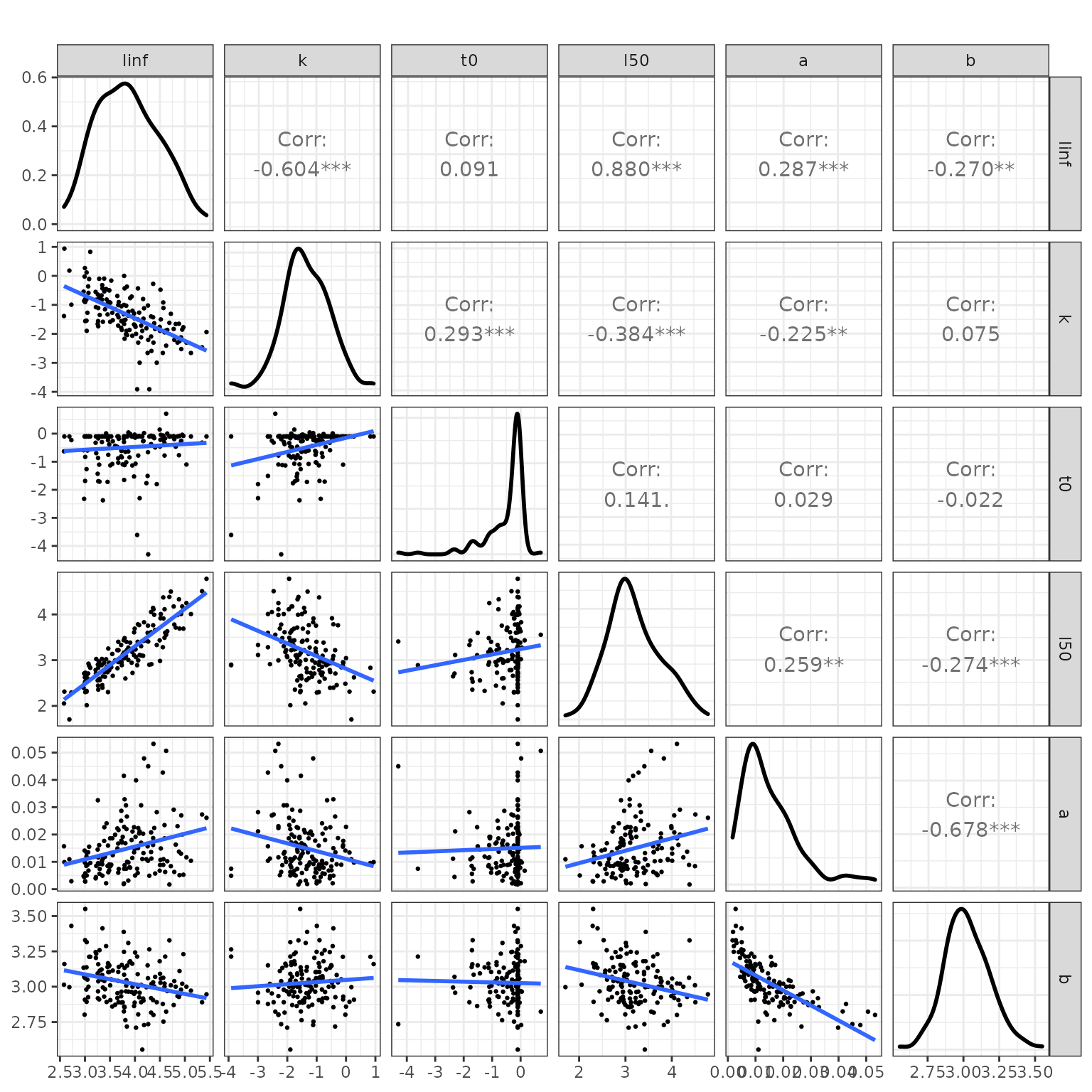
Relationship between life history parameters.
lhPar method
As seen in the above plot there are relationships between life history parameters, for example L∞ and L50 show a strong positive correlation, in other words at a a large species has a faster rate of growth than a small species.
The lhPar method can be used to fill in missing values.
Growth
Gislason, Pope, et al. (2008) proposed the relationship between k and L∞
k=3.15L−0.64∞
While Pauly (1979) proposed the empirical relationship between t0 and L∞ and k
log(−t0)=−0.3922−0.2752log(L∞)−1.038log(k)
Therefore for a value of L∞, or for the maximum observed size (Lmax ) since L∞=0.95Lmax, then missing growth parameters can be estimated.
This is done by the lhPar method, for example create an FLPar object with only linf then estimate the missing values
linf=teleost["linf"]

hat=lhPar(linf)

ggplot()+
  geom_line(aes(linf,k), data=model.frame(hat))+
  geom_point(aes(linf,k),data=model.frame(teleost),col="red")+
  scale_x_log10()+
  scale_y_log10()+
  xlab(expression(L[infinty]))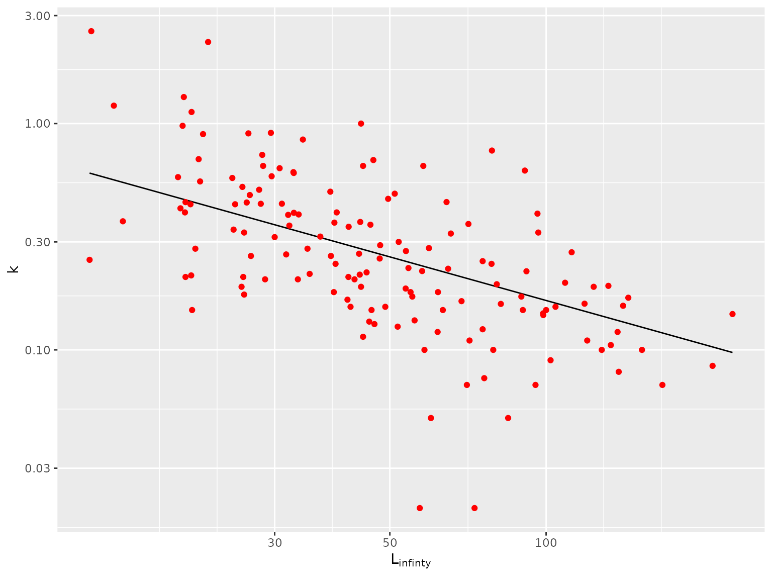
Relationship between k and Linfinty
Maturity
Beverton (1992) proposed a relationship between L50 the length at which 50% of individuals are mature
l50=0.72L0.93∞
Natural Mortality
For larger species securing sufficient food to maintain a fast growth rate entails exposure to a higher natural mortality, e.g. due to predation. While many small demersal species seem to be partly protected against predation by hiding, cryptic behaviour, being flat or by possessing spines have the lowest rates of natural mortality Griffiths and Harrod (2007). Hence, at a given length individuals belonging to species with a high L∞ may generally be exposed to a higher M than individuals belonging to species with a low L∞.
Gislason, Daan, et al. (2008) proposed the empirical relationship
log(M)=0.55−1.61log(L)+1.44log(L∞)+log(k)
Filling in missing parameters
An object of class "FLPar"
iters:  145

params
               linf                   k                  t0                   a
  45.10000(28.0211)    0.27519( 0.1218)   -1.33299( 0.0842)    0.00030( 0.0000)
                  b                 l50                 a50               ato95
   3.00000( 0.0000)   24.87234(14.4095)    1.58071( 0.9469)    1.00000( 0.0000)
               asym                  bg                  m1                  m2
   1.00000( 0.0000)    3.00000( 0.0000)    0.55000( 0.0000)   -1.61000( 0.0000)
                 m3                   s                   v                sel1
   1.44000( 0.0000)    0.90000( 0.0000) 1000.00000( 0.0000)    2.58071( 0.9469)
               sel2                sel3
   1.00000( 0.0000) 5000.00000( 0.0000)
units:  NA
Stock recruitment relationship
exportMethods(sv)
exportMethods(steepness)
lhPar assumes a Beverton and Holt stock recruitment relationship by default
R=aSSBb+SSB
Beverton and Holt (1993) as reformulated by Francis (1992) in terms of steepness (h), virgin recruitment (R0) and S/RF=0, where steepness is the rat.
R=0.8R0hS0.2S/RF=0R0(1−h)+(h−0.2)S
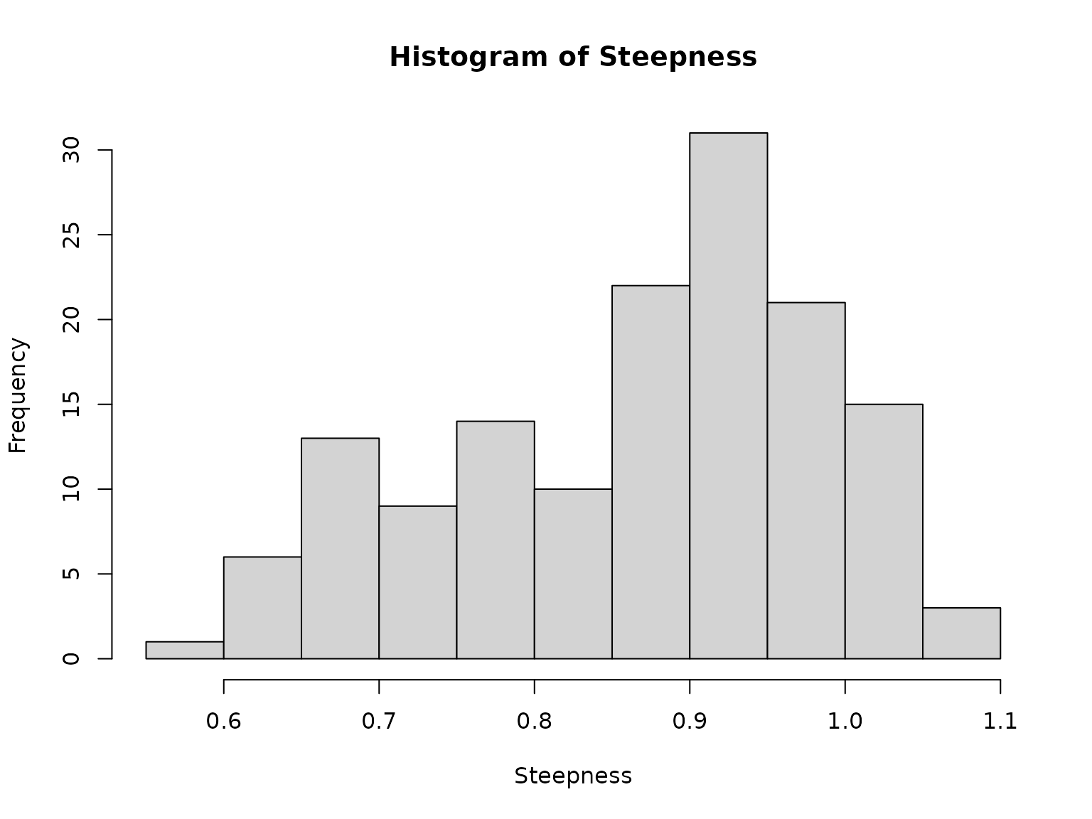
Steepness is difficult to estimate from stock assessment data sets as there is often insufficient range in biomass levels required for its estimation.
Wiff et al. (2016) investigated the relationship between life history parameters and the steepness of the stock recruitment relationship.
Logit[μi]=2.706−3.698l50/l∞ where
Logit[μi]=Logit[μi−0.21−μi]
Dynamics
Expected dynamics
Density Dependence
exportMethods(grwdd)
exportMethods(matdd)
exportMethods(mdd)
Natural Mortality
exportMethods(charnov)
exportMethods(djababli)
exportMethods(gislason)
exportMethods(griffiths)
exportMethods(lorenzen)
exportMethods(jensen)
exportMethods(jensen2) exportMethods(rikhter)
exportMethods(rikhter2)
exportMethods(petersen)
exportMethods(roff)
(???)
Nt+1=Ntexp[−M∞−Ft]1+NtAM∞+Ft{1−exp(−M∞−Ft)]}
Ct=FtAln[1+NtAM∞+Ft[1−exp(−M∞−Ft)]]
More Information
- You can submit bug reports, questions or suggestions on
FLifeat theFLifeissue page,4 or on the FLR mailing list. - Or send a pull request to https://github.com/flr/FLife/
- For more information on the FLR Project for Quantitative Fisheries Science in R, visit the FLR webpage.5
- The latest version of
FLifecan always be installed using thedevtoolspackage, by calling
    library(devtools)
    install_github("flr/FLife")
Software Versions
- R version 4.2.1 (2022-06-23)
- FLCore: 2.6.19
- FLPKG:
- Compiled: Tue Aug 30 21:12:55 2022
- Git Hash: f4ea8e3
Author information
Laurence KELL. laurie@seaplusplus.co.uk
Acknowledgements
This vignette and many of the methods documented in it were developed under the MyDas project funded by the Irish exchequer and EMFF 2014-2020. The overall aim of MyDas is to develop and test a range of assessment models and methods to establish Maximum Sustainable Yield (MSY) reference points (or proxy MSY reference points) across the spectrum of data-limited stocks.
References
- FLife-lhPar
- data
- knife
- logistic
- dnormal
- sigmoid
- FLife-m
- fapex
- lhEql
- lhRef
- lopt
- lh-indicators
- bench
- lh-srr-sv
- noise
- stars
- FLife-dd-m
- FLife-dd-mat
- grw-dd
- util
- leslie
- calcR
- len-index
- power
- spectra
- t0
- extendPlusGroup
- getScriptPath
- sim
- knifeEdgeMsy
- netSel
- funcs-indicators
- plot-bivariate
- reverse
- priors
- ggpairs
- steepness
Beverton, RJH. 1992. “Patterns of Reproductive Strategy Parameters in Some Marine Teleost Fishes.” Journal of Fish Biology 41: 137–60.
Beverton, R.J.H., and S.J. Holt. 1993. On the Dynamics of Exploited Fish Populations. Vol. 11. Springer.
Francis, R I CC. 1992. “Use of Risk Analysis to Assess Fishery Management Strategies: A Case Study Using Orange Roughy (Hoplostethus Atlanticus) on the Chatham Rise, New Zealand.” Can. J. Fish. Aquat. Sci. 49 (5): 922–30.
Gislason, H., N. Daan, JC Rice, and JG Pope. 2008. “Does Natural Mortality Depend on Individual Size.” ICES.
Gislason, H., J.G. Pope, J.C. Rice, and N. Daan. 2008. “Coexistence in North Sea Fish Communities: Implications for Growth and Natural Mortality.” ICES J. Mar. Sci. 65 (4): 514–30.
Griffiths, David, and Chris Harrod. 2007. “Natural Mortality, Growth Parameters, and Environmental Temperature in Fishes Revisited.” Canadian Journal of Fisheries and Aquatic Sciences 64 (2): 249–55.
Pauly, Daniel. 1979. “Gill Size and Temperature as Governing Factors in Fish Growth: A Generalization of von Bertalanffy’s Growth Formula.”
Wiff, Rodrigo, Juan C Quiroz, Sergio Neira, Santiago Gacitúa, and Mauricio A Barrientos. 2016. “Chilean Fishing Law, Maximum Sustainable Yield, and the Stock-Recruitment Relationship.” Latin American Journal of Aquatic Research 44 (2): 380–91.
http://www.oxfordbibliographies.com/view/document/obo-9780199830060/obo-9780199830060-0016.xml↩︎
Wilkinson, L. 1999. The Grammar of Graphics, Springer. doi 10.1007/978-3-642-21551-3_13.↩︎
http://tutorials.iq.harvard.edu/R/Rgraphics/Rgraphics.html↩︎