Sampling quantiles

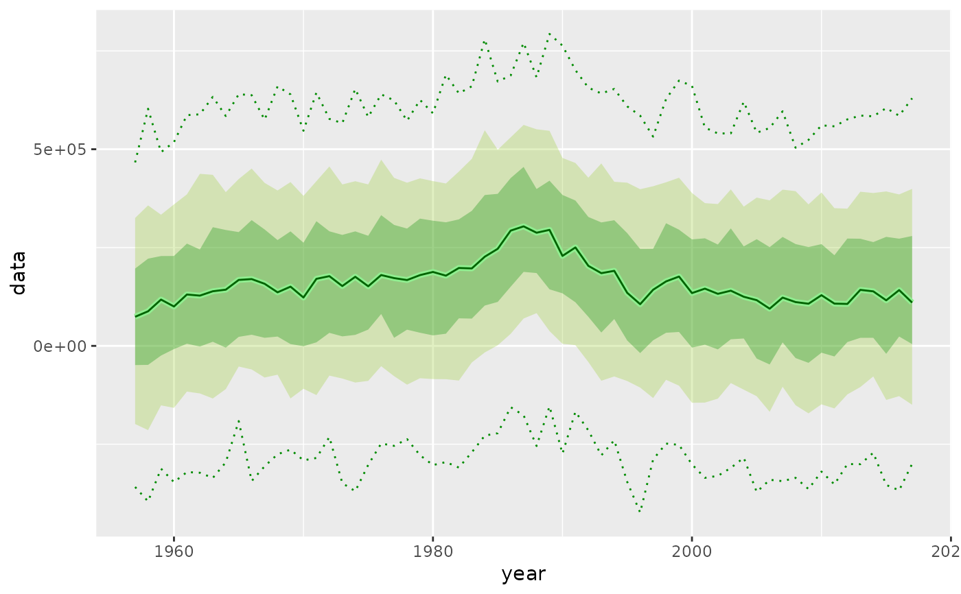
This `geom` calculates sampling quantiles and draws a ribbon for the quantile range plus a line for the median (50% quantile).

geom_flquantiles(
  mapping = NULL,
  data = NULL,
  stat = "FLQuantiles",
  position = "identity",
  show.legend = NA,
  inherit.aes = TRUE,
  na.rm = FALSE,
  probs = c(0.1, 0.5, 0.9),
  alpha = 0.5,
  ...
)

stat_flquantiles(
  mapping = NULL,
  data = NULL,
  geom = "line",
  position = "identity",
  na.rm = TRUE,
  show.legend = NA,
  inherit.aes = TRUE,
  ...
)

Arguments

mapping

Set of aesthetic mappings created by aes(). If specified and inherit.aes = TRUE (the default), it is combined with the default mapping at the top level of the plot. You must supply mapping if there is no plot mapping.

data

The data to be displayed in this layer. There are three options:

If NULL, the default, the data is inherited from the plot data as specified in the call to ggplot().

A data.frame, or other object, will override the plot data. All objects will be fortified to produce a data frame. See fortify() for which variables will be created.

A function will be called with a single argument, the plot data. The return value must be a data.frame, and will be used as the layer data. A function can be created from a formula (e.g. ~ head(.x, 10)).

stat

The statistical transformation to use on the data for this layer, either as a ggproto Geom subclass or as a string naming the stat stripped of the stat_ prefix (e.g. "count" rather than "stat_count")

position

Position adjustment, either as a string naming the adjustment (e.g. "jitter" to use position_jitter), or the result of a call to a position adjustment function. Use the latter if you need to change the settings of the adjustment.

show.legend

logical. Should this layer be included in the legends? NA, the default, includes if any aesthetics are mapped. FALSE never includes, and TRUE always includes. It can also be a named logical vector to finely select the aesthetics to display.

inherit.aes

If FALSE, overrides the default aesthetics, rather than combining with them. This is most useful for helper functions that define both data and aesthetics and shouldn't inherit behaviour from the default plot specification, e.g. borders().

na.rm

If FALSE, the default, missing values are removed with a warning. If TRUE, missing values are silently removed.

probs

Quantiles to compute and draw, defaults to c(0.10, 0.90).

alpha

Transparency for quantile ribbon.

...

Other arguments passed on to layer(). These are often aesthetics, used to set an aesthetic to a fixed value, like colour = "red" or size = 3. They may also be parameters to the paired geom/stat.

geom

The geometric object to use to display the data, either as a ggproto Geom subclass or as a string naming the geom stripped of the geom_ prefix (e.g. "point" rather than "geom_point")

Details

As this `geom` outputs two layers, although based on different `geoms`, interactions between common parameters need to be considered. The `fill` parameter will only affect the quantile range `ribbon`, but `colour` will be passed to both the `ribbon` and median `line` layers. The defaults are no lines on the quantiles and "black" for the median line. The `alpha` value has been hard coded to 1 for the median line, so only affects the quantile `ribbon`. To change this, call `stat_flquantiles` directly, as in the examples below.

`stat_flquantiles` will return between one and three `y` values depending on the number of quantiles requested. If two quantiles are to be calculated, it will return the corresponding `ymin` and `ymax`, to be used with, for example, `geom_ribbon`. If only one quantile is to be calculated, it will be returned as `y`, to be used typically by `geom_line`. Finally, if three values are passed in the `probs` argument, all of the above will be returned, in the right order.

Aesthetics

`geom_flquantiles` understands the following aesthetics (required aesthetics are in bold): - `*x*` - `*y*` - `alpha` - `colour` - `fill` - `group` - `linetype` - `linewidth` where some of them apply to the ribbons and some of them to the lines.

Computed variables

y

quantile, if only one requested or central one when if three

ymin

lower quantile, if two or three requested

ymax

upper quantile, if two or three requested

Examples

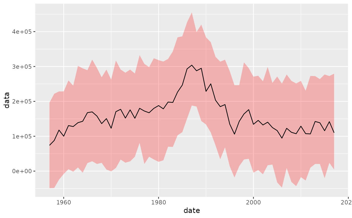
data(ple4)
flq <- rnorm(250, catch(ple4), 200000)
ggplot(flq, aes(x=date, y=data)) +
  geom_flquantiles(probs=c(0.25, 0.50, 0.75), fill="red", alpha=0.25)

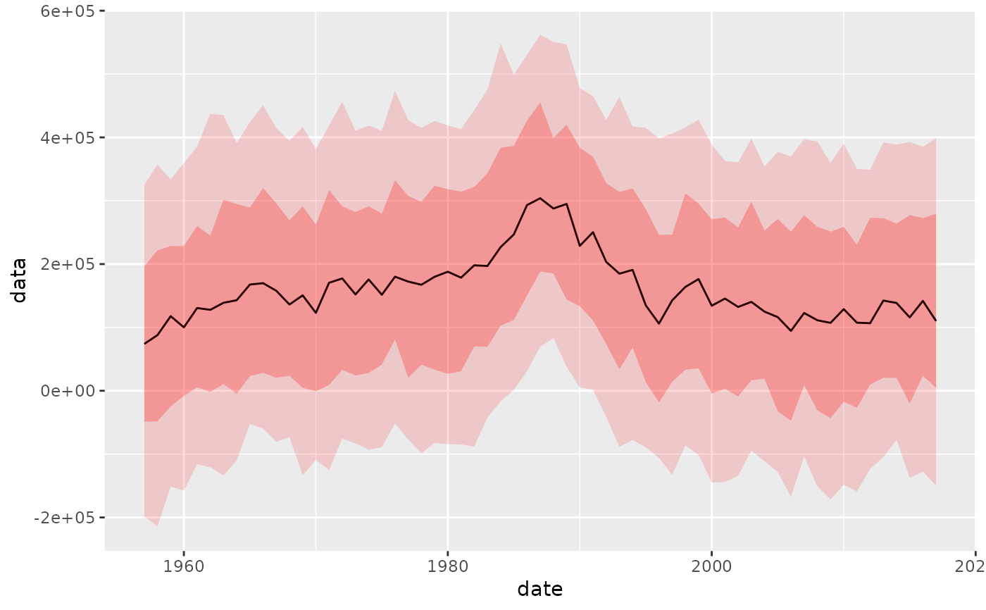
# Draw two quantiles with two calls to geom_flquantiles
ggplot(flq, aes(x=date, y=data)) +
  geom_flquantiles(probs=c(0.25, 0.50, 0.75), alpha=0.25, fill="red") +
  geom_flquantiles(probs=c(0.10, 0.90), alpha=0.15, fill="red")

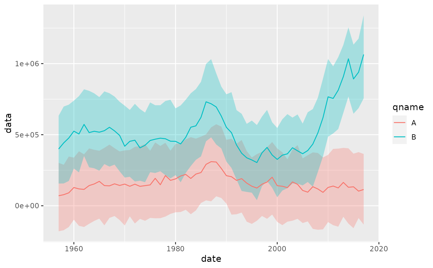
# Use it on an FLQuants, colouring by their name
flqs <- FLQuants(A=rnorm(250, catch(ple4), 200000),
  B=rnorm(250, stock(ple4), 200000))
ggplot(flqs, aes(x=date, y=data, colour=qname)) +
  geom_flquantiles(probs=c(0.10, 0.50, 0.90), aes(fill=qname), alpha=c(0.30))

# Or facet them
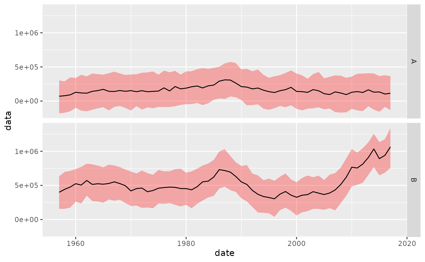
ggplot(flqs, aes(x=date, y=data)) +
  geom_flquantiles(probs=c(0.10, 0.50, 0.90), fill="red", alpha=c(0.30)) +
  facet_grid(qname~.)

# For greater control, call stat_flquantiles directly with a geom
ggplot(flq, aes(x=year, y=data)) +
 stat_flquantiles(probs=c(0.10, 0.90), geom = "ribbon",
   fill="yellowgreen", alpha=0.30) +
 stat_flquantiles(probs=c(0.01), geom = "line",
   colour = "green4", linetype=3) +
 stat_flquantiles(probs=c(0.99), geom = "line",
   colour = "green4", linetype=3) +
 stat_flquantiles(probs=c(0.25, 0.75), geom = "ribbon",
   fill="green4", alpha=0.30) +
 stat_flquantiles(probs=c(0.50), geom = "line", linewidth=1.5,
   colour = "lightgreen") +
 stat_flquantiles(probs=c(0.50), geom = "line",
   colour = "darkgreen")